MossWinn 4.0 series help

• Contact:

• e-mail: z.klencsar@mosswinn.hu
• web: http://www.mosswinn.com, http://www.mosswinn.hu

• To read this Help:

• The web browser Mozilla Firefox is recommended.
• Increase / decrease font size by pressing ctrl + / ctrl -

The main menu is the root of the menu system of the MossWinn program. This is the menu that appears on start up. It provides access to numerous other menus and functions mainly via the menu boxes arranged in two blue colored side-menu columns on the left and right hand side of the screen, as well as via responding to keyboard keypress events. The program can be closed by clicking on the Exit menu box in the right bottom corner of the screen. Closing is immediate, it can not be cancelled. When next time the program is executed, it will continue where it left off.

• The function of the menu boxes - click on the menu box of interest. (Depending on the state of the program some menu boxes may appear grayed out indicating that the corresponding menu is not available for the actual state.)

• Applicable keystrokes

• F1 - Set application window such that its size (in pixels) corresponds to 1x the internal MossWinn screen resolution.
• F2 - Set application window such that its size (in pixels) corresponds to 2x the internal MossWinn screen resolution.
• F3 - Set application window such that its size (in pixels) corresponds to 3x the internal MossWinn screen resolution.
• F4 - Toggle between full screen and windowed modes.
• F5 - Toggle between always on top and normal window modes.
• F8 - Show or hide the edit spectrum parameters dialog.

• F12 - Invoke this help file.

• TAB - Go to the next active project desk.
• Backspace - Go to the previous active project desk.

• E - Edit the text file associated with the red-framed window by executing the user-defined editor program (see the EXE menu).
• ESC - Show/hide the blue side menus. (Rearranges the spectrum windows.)

• ctrl-C - Copy image of the red-framed spectrum into the clipboard of Windows.
• ctrl+shift-C - Copy image of all the spectra on the screen into the clipboard of Windows.
• ctrl-P - Print image of the red-framed spectrum to the default Windows printer.
• ctrl+shift-P - Print image of all the spectra on the screen to the default Windows printer.

• J - Save image of the red-framed spectrum as a JPEG image file.
• shift-J - Save image of all the spectra on the screen as a JPEG image file.
• C - Save image of the red-framed spectrum as a 24 bit color bitmap.
• shift-C - Save image of all the spectra on the screen as a 24 bit color bitmap.
• B - Save image of the red-framed spectrum as a 1 bit B&W bitmap.
• shift-B - Save image of all the spectra on the screen as a 1 bit B&W bitmap.

• R - to show/hide the residual for the red-framed spectrum window.
• shift-R - to show/hide the residual for all the spectrum windows.

• shift-M - Display the amount of physical memory available to MossWinn.
• shift-A - Display the 'About' page of MossWinn.

• The popup menu of data windows - the popup menu list of a data window is invoked by a mouse click on its - cyan colored - headline. The menu list provides the following options concerning the selected window:

• Open HTML FitLog - to open the HTML FitLog file that contains fit reports logged previously in the FIT menu for the spectrum in the selected window. The FitLog file is opened in the default web browser application.

• Create copy - to create an independent copy of the window and the associated data file. The newly created data file copy is placed inside the host directory of the orginal, and is given a name that differs from that of the original by numbering.
• Create temporary copy - to create an independent temporary copy of the window and the associated data file. The newly created data file copy is placed inside the temporary directory of MossWinn, and is given a name that has the extension of TMP. By 90 days after their creation, temporary files are moved to the trash directory of MossWinn without notice. Windows associated with temporary files are denoted by a lightgray - rather than blue - frame in MossWinn.

• Rename associated file - to rename the file associated with the selected window.
• Update on disk - to update the content of the file associated with the selected window according to the actual state of the window. If the window does not have an associated file (i.e. it has not been saved yet), then it will be saved as a temporary file.
• Reload from disk - to reload the content of the selected window from the file associated with it.

• Copy as xls - to make a copy of the spectrum data in the selected data window in the form of an XLS spreadsheet file (example). Once created, MossWinn attempts to open the XLS file with an associated software application. Access to this option requires subscription to the MossWinn Services. For further details click here.
• Print to printer - Print image of the selected data window either to the default, or to the selected printer.
• Copy to clipboard - Copy image of the selected data window into the clipboard of Windows.
• Copy to clipboard (as text) - Copy the spectrum data associated with the selected window into the clipboard of Windows as text, including the velocity axis, the measured data, the fit envelope and the subspectra in separate columns as comma delimited numerical data. This option may be used to export numerical data from MossWinn to external graphics software.

• Show residual - to show/hide the residual for the selected data window.
• Recalibrate Y axis - to adjust the Y axis scale such that all relevant data points are visible.
• Consider/Ignore zero data points - to consider/ignore zero valued data points when displaying, fitting, etc. of the selected spectrum. Normally, zero valued data points are ignored, i.e. they are regarded as 'bad points' not to be considered when the spectrum is displayed, fitted or manipulated in any other way.

• Add to headline content - to make the selected item to be displayed in the headline of the selected window.
• Remove from headline content - to make the selected item not to be displayed in the headline of the selected window.
• Set current as default headline content - to make the actual headline content to be the default one concerning the items to be displayed. This will influence the window headline of spectra newly loaded/encountered by MossWinn.

• The meaning of different window frame colors - the main menu displays the various windows with different frame colors.

• Red window frame - The red (i.e. red-framed) window is the master/target window, that is, any selected operation gets carried out on the spectrum in this window. Unless the current desk is empty, there is always exactly one master window on the screen. To make a blue-, gray- or green-framed window to be the master window, press on it with the left mouse button. In order to have the red window display information on the corresponding data, press on it with the left mouse button. A further press on it will make it display the spectrum graph again.
• Blue window frame - The default color of a window (-frame) is blue.
• Green window frame - The green (i.e. green-framed) window takes the role of the source window in various operations that are performed on the red-framed (target) window. For example, the data in the green window can be subtracted from the data of the red window by a press on the SBC menu box, the FIT menu is entered for the red window by taking the fit model from the green window, etc.
• Gray window frame - Windows referring to files inside the temporary directory of MossWinn are displayed with a gray frame unless selected to be red- or green-framed. (Concerning the creation of temporary files, see above.)

The Load menu box

• Accessible from the Main menu.

• Functions:

• Left mouse button - to enter the LOAD / Data Input menu.
• Right mouse button - to display the Load File Windows Dialog.

The ARR menu box

• Accessible from the Main menu.

• Functions:

• Left mouse button - to arrange the displayed - data and text - windows in rows & columns.
• Right mouse button - to display the menu list of special arrange functions that provide the possibility to arrange the windows in an increasing order with respect to one of the default or user-defined special parameters.

The SRE menu box

• Accessible from the Main menu.

• Function:

• Left/right mouse button - to enter the SRE (Spectrum Recovery) menu, which provides the possibility to manipulate measured data counts especially in order to fix spectrometer overflows and faults (e.g. dropped-down data points). The menu becomes activated for the red-framed spectrum window.

The FLD menu box

• Accessible from the Main menu.

• Function:

• Left/right mouse button - to display the FLD (Fold) dialog, that provides the possibility to fold unfolded spectra either at the folding point determined automatically, or at a folding point set by the user manually. Changing the minimum or maximum value of the folding point will result in a recalculation of the recommended (automatically determined) folding point. The dialog becomes activated for the red-framed spectrum window, whereas the resulting, folded spectrum appears in a new window. The folded spectrum is saved automatically inside the host directory of the original, unfolded spectrum. The extension of the saved file will be changed to the extension that can be set by the user in the SET menu list.

The REV menu box

• Accessible from the Main menu.

• Function:

• Left/right mouse button - to carry out the reverse operation on the red-framed spectrum. The resulting new spectrum - placed in a new window - will contain exactly the same data as the original spectrum did, but in reversed order. If the original spectrum is calibrated according to a linear scale, then on reversion the calibration constant zero velocity channel is modified as well, such that the counts belonging to the zero velocity remains unchanged. The reversed spectrum is saved automatically inside the host directory of the original spectrum. The extension of the saved file will be changed to the extension that can be set by the user in the SET menu list.

The CAL menu box

• Accessible from the Main menu.

• Functions (in the absence of any green-framed spectrum window):

• Left mouse button - to display the CAL (Calibration) dialog, that provides the possibility to calibrate the red-framed spectrum according to a linear scale by setting the calibration factor and zero velocity channel calibration constants.
• Right mouse button - to display the CAL (Calibration) dialog, that provides the possibility to calibrate the red-framed spectrum according to a linear scale by setting the calibration factor and velocity of the first channel calibration constants.

• Function (in the presence of a suitable green-framed spectrum window):

• Left/right mouse button - to transfer calibration information from the green-framed spectrum to the red-framed one. If the operation is successful, the velocity axis of the red-framed spectrum will be identical to that of the green-framed one. This is the usual way to transfer calibration information from an already calibrated spectrum (e.g. that of alpha iron) to a spectrum measured with the same velocity settings. (To make a blue-framed spectrum window turn green-framed or vice versa, click on it with the right mouse button.)

The ASP menu box

• Accessible from the Main menu.

• Functions (in the presence of a suitable green-framed spectrum window):

• Left mouse button - to apply the same FLD (fold), REV (reverse) and CAL (calibration) operations (as they were applied earlier to the green-framed spectrum) to the red-framed spectrum. The result is saved automatically inside the host directory of the original spectrum.
• Right mouse button - to apply the same FLD (fold), REV (reverse) and CAL (calibration) operations (as they were applied earlier to the green-framed spectrum) to all but the green-framed spectrum. The results are saved automatically inside the respective host directories of the original spectra.

The PLT menu box

• Accessible from the Main menu.

• Functions:

• Left mouse button - to change the appearance of the red-framed window or of all the windows at once:

• Apply to all - to apply the selected option to all the windows on the current desk.
• Consider/Ignore zero points - to consider/ignore zero valued data points when displaying, fitting, etc. of the red-framed spectrum. Normally, zero valued data points are regarded as 'bad points' not to be considered when the spectrum is displayed, fitted or manipulated in any other way. 'Fixing' data in the SRE menu also means that the value of the selected data points are set to zero.
• Show/Hide horizontal line at Y=0.0 - to show/hide a horizontal line at the ordinate value of Y=0.0 in the red-framed data window. If the Y axis range does not contain the value of Y=0.0, then the line won't appear. This option is useful e.g. for inspecting residuals created via the SBC menu box.
• Point size... - to select Auto/Large/Small data point size for the red-framed spectrum window. When Auto is selected, the program chooses between Large and Small point sizes depending on the size of the window.
• Connect/Disconnect points - toggle between scatter and line graph modes for the red-framed spectrum window.
• Show/Hide StD bars - to show/hide StD bars for the red-framed spectrum window. StD bars extend ±σ around the data points where σ is the square root of the data count value. When StD bars are shown, the data points are displayed disconnected from each other.
• Show/Hide residual - to show/hide the residual for the red-framed spectrum window. The residual is calculated by subtracting the red fitting envelope from the measured data, then it is shifted to be positioned above the spectrum data. A magenta-colored horizontal line denotes the zero level of the residual, while a grey stripe indicates (approximately) the levels of +1 Std and -1 Std around the zero level. The residual is visible only if the spectrum window contains a fitting envelope.
• Show/Hide Y axis - to show/hide the Y (vertical) axis of the red-framed spectrum window.
• Use/Hide suffix - to use/hide suffix notation in the numerical labels of the Y axis of the red-framed spectrum window. Suffix notations include k (kilo, 10³), M (Mega, 10⁶), G (Giga, 10⁹), T (Tera, 10¹²), P (Peta, 10¹⁵) and E (Exa, 10¹⁸). On graphical outputs the suffix notations appear as a /10ⁿ extension after the Y axis title.
• Show percentage/absolute values - toggle between percentage (i.e. relative) and absolute numerical representation of the Y (ordinate) values in the red-framed spectrum window. In percentage representation the ordinate values are meant relative to the (signed) maximum of the data, y_i(%)=100*(y_i/y_max). (According to the above, for negative valued data the percentage representation may result in values lower than -100%).
• Transparent/Not transparent - to make the red-framed window transparent/not transparent. In transparent mode the white background of the window is not drawn, such that windows being below the transparent window can be seen as well.
• Ungroup window - to create a separate data window for all or only one of the fitting envelops being present in the red-framed spectrum window. To create a separate window for all of the fitting envelops, click directly on this item, whereas to create a separate window only for a single fitting envelope, select one of them in the appearing list.
• Group with green - to add all the data series being part of the green-framed spectrum window to the red-framed spectrum window. In the red-framed window the newly added data series will appear as additional fitting envelops. Fitting envelops can be removed from a data window via the menu list of the DEL menu box (accessible by a click with the right mouse button).
• Make a copy of red - to create an independent copy of the red-framed data window.

• Right mouse button - toggle between scatter and line graph modes for the red-framed window. Scatter graph mode can be activated only for the measured data, fitting curves are always displayed in line graph mode.

The EDT menu box

• Accessible from the Main menu.

• Function:

• Left mouse button (equivalent to the F8 key) - to display the Edit Spectrum Parameters Dialog that enables one

• to set the value of various spectrum parameters for the red-framed window - the value of parameters such as the stoichiometry and temperature of the sample, further experimental parameters and keywords associated with the corresponding measurement, and the headline of the associated spectrum file can be set here among others (example).
• to monitor the last accepted fit results associated with the red-framed window - the complete fit report (if available) can be displayed, printed or copied to clipboard (example). (Use the mouse wheel or press with the left mouse button to scroll the fit report content. The dialog can also be resized to see more of the fit report at once.)
• to monitor the fitness of models in related MIDB database records with respect to the spectrum in the red-framed window - move the mouse pointer over any of the displayed (related) MIDB database records (under the MIDB matches tab) to evaluate the fitness of the corresponding model with respect to the spectrum in the red-framed window (example 1, example 2). MIDB records (selected either from all of the records or exclusively from own records) are listed here in the order of their fitness concerning the sample stoichiometry and the selected experimental parameters. In the absence of records with good fitness, it may happen that no record is shown.
• to set the fit model of a related MIDB database record as the fit model accepted for the spectrum in the red-framed window - double-click on any of the displayed records in order to accept the corresponding model for the spectrum in the red-framed window. As a result, when next time the FIT menu is entered for the given spectrum window, the fit will start with the model accepted here.

• Right mouse button - to set a certain spectrum parameter (e.g. Stoichiometry) to the same value for all the data windows on the current project desk.

The ART menu box

• Accessible from the Main menu.

• Function:

• Left/right mouse button - to carry out arithmetical operations on the red-framed spectrum data, and to place the obtained result in a separate data window (the data in the original, red-framed window will remain unaffected):

• Multiply by a constant - to multiply each data value in the red-framed data window by the same constant, and place the result in a new data window.
• Multiply RED by GREEN - to multiply each data value in the red-framed data window by the respective data value in the green-framed data window, and place the result in a new data window. Note that this operation disregards the calibration of the X (velocity) axis.
• Normalize spectrum - to normalize the red-framed spectrum and place the result in a new window. Normalization is based on an estimated base line value (BL) that can be overruled by the user. The normalized spectrum is calculated as Y_i(normalized)=MAX(BL-Y_i,0)/MAXIMUM_k(BL-Y_k), where MAX(a,b) denotes a if a>b and it denotes b otherwise, whereas MAXIMUM_k(a_k) denotes the maximum of a_k considering all possible values of k. Consequently, the Y (ordinate) values of the normalized spectrum will all lie in the range of [0,1]. Normalization does not work for negative valued data sets.
• Divide by a constant - to divide each data value in the red-framed data window by the same constant, and place the result in a new data window.
• Divide RED by GREEN - to divide each data value in the red-framed data window by the respective data value in the green-framed data window, and place the result in a new data window. Note that this operation disregards the calibration of the X (velocity) axis.
• Strip data... - to strip off the selected subspectrum envelope curve from the measured data in the red-framed spectrum window, and place the result in a new data window. The stripped spectrum is calculated as
  
  Y_i(stripped) = Y_i - Y_i[SUB]+MAXIMUM_k(Y_k[SUB]) (for transmission spectra) and
  
  Y_i(stripped) = Y_i - Y_i[SUB]+MINIMUM_k(Y_k[SUB]) (for scattering - e.g. CEMS - spectra),
  
  where [SUB] refers to the subspectrum stripped off.
• Set minimum to zero - to subtract the minimum of the data in the red-framed data window from every data value of the window, and place the result in a new data window.
• Set negative to zero - to set all the negative valued data in the red-framed data window to zero, and place the result in a new data window.
• Set negative to positive - to take the absolute value of the data in the red-framed data window, and place the result in a new data window.
• Horizontal reflection of data - to turn absorption peaks into emission peaks and vice versa for the red-framed spectrum window, and place the result in a new data window. The transformation is carried out as Y_i(transformed)=MAXIMUM_k(Y_k)-Y_i+MINIMUM_k(Y_k). (Note that applying the transformation twice will give back the original spectrum.)
• Set zeros equal to red envelope - to set zeroed data equal to the corresponding value of the red fitting envelope of the red-framed spectrum. This option can be used to eliminate bad/zeroed data points after the spectrum was satisfactorily fitted in the FIT menu, which may prove to be useful when one exports the corresponding spectrum data to an external grapher software.
• Convolution with a Gaussian - to convolve the data in the red window with a Gaussian curve, and place the result in a new data window. The convolution is carried out simply by adding up Gaussian curves with appropriate weight factors:
  
  Y_k(result) = SUM_j(Y_j*Gaussian(v_j,v_k))
  
  where Gaussian(v_j,v_k) denotes the value of a Gaussian function centered at v_j and having an area of 1, as calculated for the abscissa of v_k. The width (FWHM) of the Gaussian is defined by the user.
• Convolution with a Lorentzian - to convolve the data in the red window with a Lorentzian curve, and place the result in a new data window. The convolution is carried out simply by adding up Lorentzian curves with appropriate weight factors:
  
  Y_k(result) = SUM_j(Y_j*Lorentzian(v_j,v_k))
  
  where Lorentzian(v_j,v_k) denotes the value of a Lorentzian function centered at v_j and having an amplitude of 1, as calculated for the abscissa of v_k. The width (FWHM) of the Lorentzian is defined by the user.
• Add normally distributed noise - to add normal statistical noise to the data in the red-framed window by assuming that for a given data the variance of the noise distribution and the value of the data are equal (referring to the underlying Poisson distribution), and place the result in a new data window.
• Add noise with fixed variance - to add normal statistical noise to the data in the red-framed window by assuming that the variance of the noise probability distribution is the same for all data points, and place the result in a new data window. The value of the uniform variance is defined by the user.
• Recover original baseline - to estimate and recover the original baseline of a spectrum that was obtained by dividing the measured spectrum data by a constant factor (e.g. the baseline itself). In order to recover the baseline value of a spectrum that was normalized in this way, it has to be fitted to some model previously, so that the red envelope of the fit estimates well the measured data. Then select this option to calculate and place the spectrum with the recovered baseline in a new window.
• Recover original baseline (in case of overflows) - to estimate and recover the original baseline of a spectrum that was obtained by subtracting a constant from the spectrum data (this happens, e.g., during overflows). In order to recover the baseline value of a spectrum, it has to be fitted to some model previously, so that the red envelope of the fit estimates well the measured data. Then select this option to calculate and place the spectrum with the recovered baseline in a new window.
• Shift velocity axis... - to add a certain (positive or negative) constant to the velocity value of each channel of the spectrum in the red-framed window, and place the result in a new data window. By the use of this option one can modify the calibration of the velocity axis. For example, in order to transform a calibration relative to alpha iron to a calibration relative to Stainless Steel (SS), one would add IS (isomer shift of alpha-Fe relative to SS) = + 0.09 mm/s to the velocity value of each channel.
• Restrict velocity axis... - to restrict the velocity axis (either only of the spectrum in the red-framed window or of all spectrum windows on the current desk) to a velocity range to be defined by the user as [v_min...v_max] on the appearing dialog. The resulted spectra are placed in new windows, while the original spectra (and the corresponding files) remain unaltered. The number of channels in the processed spectrum copies will be changed in accordance with the user-defined velocity interval.
• Shift subspectra for graphics... - to display the Subspectrum Shifter Dialog that enables the manual vertical shifting of the subspectra and the residual with respect to the measured data in order to create a dataset with a clear visualization of the shape and position of subspectra. The residual appears here as if it was one of the subspectra. The menu is also useful to create a visually attractive format of the fitted spectrum data for the creation of spectrum graphics in external graphics software.

The ADD menu box

• Accessible from the Main menu.

• Functions (in the presence of a suitable green-framed spectrum window):

• Left/right mouse button - to add the spectrum in the green-framed window to the spectrum in the red-framed one, and place the result in a new data window. The addition of two spectra is possible only if their velocity axis is identical (same amount of channels, identical calibration).

• Functions (in the absence of a suitable green-framed spectrum window):

• Left mouse button - to add a constant value to every channel of the red-framed spectrum, and place the result in a new data window.
• Right mouse button - to add up neighboring channels of the red-framed spectrum, and place the result in a new data window. In the case of linearly calibrated spectra the calibration constants are modified as:
  
  CF(result) = 2*CF(original), ZVC(result) = ZVC(original)/2
  
  where CF and ZVC denote the calibration factor and the zero velocity channel, respectively.

The SBC menu box

• Accessible from the Main menu.

• Functions (in the presence of a suitable green-framed spectrum window):

• Left/right mouse button - to subtract the spectrum in the green-framed window from the spectrum in the red-framed one, and place the result in a new data window. The subtraction of the spectra from each other is possible only if their velocity axis is identical (same amount of channels, identical calibration).

• Functions (in the absence of a suitable green-framed spectrum window):

• Left mouse button - to subtract a constant value from every channel of the red-framed spectrum, and place the result in a new data window.
• Right mouse button - to calculate the residual of the red-framed spectrum, and place the result in a new data window. The residual is calculated by subtracting the red fitting envelope from the measured (black colored) data in the red-framed window. This option is available only if the red-framed window contains a fitting envelope.

The SET menu box

• Accessible from the Main menu.

• Function:

• Left/right mouse button - to display the SET menu list that allows the setting of various configuration options of MossWinn:

• Set user title, name and contact - to set the title, name and E-mail that identify you when you publish data in the MossWinn Internet Database. It is recommended that you give your real name and E-mail here, like in the example below.
• User title: Dr.
• User name: Zoltán Klencsár
• User contact: z.klencsar@mosswinn.hu
• Set internet access options - to enable/disable internet access related functions. Note that some internet functions can also be invoked manually via the Help menu.
• Automatically download updates of the MossWinn manual. [ Enabled ]
• Automatically download updates of MossWinn help files. [ Enabled ]
• Automatically check for updates of MossWinn executables. [ Enabled ]
• MossWinn Internet Database (MIDB) access. [ Enabled ]
• Set performance options... - to set options influencing various aspects of the performance of MossWinn, e.g. whether MossWinn is allowed to utilize its parallel computing routines to speed up the corresponding calculations on multi-core processor systems.
• Parallel computation on multiple cores [ Enabled ] - set it to enabled to allow MossWinn to engage its parallel computing algorithms on multicore-processor systems.
• Automatic HTML FitLog creation on Accept [ Enabled ] - set it to enabled to allow MossWinn to log automatically a HTML fit report to the FitLog file associated with the spectrum under fitting, when the fit is accepted (by pressing with the left mouse button on the Accept menu box) in the FIT menu.
• Inclusion of related database links into FitLogs [ Enabled ] - set it to enabled to allow MossWinn to include into HTML FitLogs (DOI based) publication links from MIDB database records that report about measurements of materials with a stoichiometry that is similar to that associated with the fitted spectrum (example). This function works only when the MIDB database service is accessible.
• Resolution of spectrum images in HTML FitLogs [ LOW / MEDIUM / HIGH ] - set to determine the resolution of fitted spectrum images included in HTML FitLog files. The options are LOW (640×480), MEDIUM (800×600) and HIGH (1024×768).
• Enable/disable libraries - to enable the loading and calling of those dynamic link libraries that one intends to use for the calculation of the corresponding subspectrum curve(s) in the FIT menu. The libraries in question should have a file name corresponding to the mask SUB*.DLL, and they should be present in the code library directory of MossWinn.
• Set mouse type... - to set whether the mouse is to be treated as a left-handed or as a right-handed mouse. When in Windows the function of the left and right mouse buttons are swapped, then MossWinn will start by assuming a left-handed mouse. Setting the mouse to be left-handed or right-handed in MossWinn will not alter the corresponding (system-wide) setting in Windows.
• Left-handed - if the mouse is set to be left-handed, then the functions attributed to the left and right mouse buttons are swapped (compared to what is described in this help).
• Right-handed - if the mouse is set to be right-handed, then the left and right mouse buttons function as described in this help.
• Set color scheme... - to alter the default colors used by MossWinn, which can help to improve perceived color differences of the main MossWinn screen.
• Default color scheme - to restore the default color scheme of MossWinn.
• Create color scheme... - to display the form that allows one to create and save a new, alternative color scheme for MossWinn.
• Delete current color scheme - to delete the currently set alternative color scheme.
• Set GUI resolution... - to alter and check on the internal MossWinn GUI (graphical user interface) screen resolution.
• 640 x 350 - to set the internal MossWinn screen resolution to 640 x 350 (width x height) which was the internal resolution of the MossWinn screen in MossWinn versions from 1.0 to 4.0 .
• 640 x 400 - to set the internal MossWinn screen resolution to 640 x 400.


• 800 x 400 - to set the internal MossWinn screen resolution to 800 x 400.
• 800 x 450 - to set the internal MossWinn screen resolution to 800 x 450.
• 800 x 500 - to set the internal MossWinn screen resolution to 800 x 500.
• 800 x 650 - to set the internal MossWinn screen resolution to 800 x 650.
• 900 x 450 - to set the internal MossWinn screen resolution to 900 x 450.
• 900 x 500 - to set the internal MossWinn screen resolution to 900 x 500.
• 900 x 650 - to set the internal MossWinn screen resolution to 900 x 650.


• Set optimum resolution for full screen mode - to set the internal MossWinn screen resolution equal to a value that is optimum for full screen mode by considering the full resolution of the current screen.
• Set optimum resolution when entering full screen mode - when selected, the internal MossWinn screen resolution is automatically set to be equal to a value that is optimum for full screen mode whenever the latter is entered by pressing F4. When full screen mode is entered with this option being unselected, the program sets the internal resolution to the one last used in full screen mode.


• 960 x 540 (Optimum for FHD full screen) - to set the internal MossWinn screen resolution to 960 x 540, which is considered to be optimum in full screen mode on a FHD (1920 x 1080) screen.
• 960 x 600 (Optimum for WUXGA full screen) - to set the internal MossWinn screen resolution to 960 x 600, which is considered to be optimum in full screen mode on a WUXGA (1920 x 1200) screen.
• 1280 x 540 (Optimum for UW-UXGA full screen) - to set the internal MossWinn screen resolution to 1280 x 540, which is considered to be optimum in full screen mode on an UW-UXGA (2560 x 1080) screen.
• 1280 x 720 (Optimum for QHD & 4K HD full screen) - to set the internal MossWinn screen resolution to 1280 x 720, which is considered to be optimum in full screen mode on QHD (2560 x 1440) and 4K HD (3840 x 2160) screens.
• 1720 x 720 (Optimum for UW-QHD full screen) - to set the internal MossWinn screen resolution to 1720 x 720, which is considered to be optimum in full screen mode on an UW-QHD (3440 x 1440) screen.
• 1920 x 1080 (Alternative for FHD and 4K HD full screen) - to set the internal MossWinn screen resolution to 1920 x 1080, which is considered as a higher resolution alternative on FHD (1920 x 1080) and 4K HD (3840 x 2160) screens.


• Set maximum resolution for full screen mode - to set the internal MossWinn screen resolution to its maximum value considering the full resolution of the current screen. This option is available only when the program is in full screen mode.


• Set ASCII keyboard layout - to display the Customize ASCII keyboard layout dialog that can be used to redefine character inputs in which keystrokes result in MossWinn. When the dialog is displayed, press a key (or shift + key) and then, by using the mouse, in the ASCII list select the character in which the pressed key should result in when entered in MossWinn. Select Restore to invalidate all changes and restore the default layout.
• Set autosave options... - to set the file extensions used when spectra are automatically saved by MossWinn, as well as to set the frequency by which the status of the fit menu is saved during fitting.
• On fold spectra (FLD) [ FLD ]
• On reverse spectra (REV) [ DAT ]
• On auto-copy of original data files (ENABLED) [ MOS ]
• Autosave fit status [ ... ]
• Set default calibration options... - to set the default attributes of calibration spectra:
• 57Co source matrix (rhodium, chromium or palladium)
• Calibration material (e.g. Alpha Iron)
• Isomer shift reference (e.g. Alpha Iron)
• Default graphics font... - to set the font that is used when graphical images of spectra are printed to printer, saved to file or copied into the clipboard:
• Arial
• Cambria
• Triplex
• Times New Roman.
• Default printer to be used... - to set the Windows printer that is used when text or graphics is printed by MossWinn.
• Page orientation when printing... - to set the default page orientation (portrait or landscape) when graphics is printed by MossWinn.
• Special parameters... - to define, delete or set the value of special parameters.
• Define new special parameter type
• Delete existing parameter type
• Set special parameter values for the red window
• Configuration settings... - to check on and to set of various options initially offered for setting when MossWinn was installed.
• Edit configuration file... - to directly edit the content of one of the configuration files, by invoking either the text editor program selected in the EXE menu, or the system's default text editor program (in the case of EDITPROG.CFG).
• Reload configuration files - to reload all configuration files in order to make MossWinn aware of their actual state. This option is useful especially after one has directly edited the content of some configuration file and wants the changes to take effect without restarting MossWinn. Normally, configuration files are loaded only when MossWinn starts up.

The DEL menu box

• Accessible from the Main menu.

• Functions:

• Left mouse button - to delete the red-framed window from the current project desk. On delete the window is moved to the Trash desk of the current project group. Windows on the Trash desk can be reloaded by clicking with the right mouse button on the DEL menu box. Deleting a window from a project desk does not influence the corresponding physical file whose content the window displays.

• Right mouse button - to display the menu list of special delete functions:

• Delete all windows on all of the desks - to delete all the - data and text - windows loaded in MossWinn. This will make all active project desks empty. With the exception of the General Projects . General Desk and the Trash desks, empty project desks do not get updated on closing the program.
• Delete all windows on the current desk - to delete all the - data and text - windows loaded in MossWinn on the current desk.
• Unload from memory all desks but current - to make the actually displayed desk to be the only one that is active. When a new project desk is selected, then the old one may remain in memory, i.e. it may remain active. There can be a maximum of 16 active project desks loaded in MossWinn. Press the TAB and Backspace keys to navigate (i.e. go forward and backward, respectively) among the active project desks.
• Delete text windows - to delete all text windows (i.e. windows whose content is not interpreted/displayed as a function of numerical data) on the current project desk.
• Delete blue-framed windows - to delete blue-framed windows on the current project desk.
• Delete gray-framed (temporary) windows - to delete gray-framed windows that, on the current project desk, display the content of data files located in the temporary directory of MossWinn.
• Delete invisible windows on the current desk - to delete those windows on the current project desk that are fully covered by other windows.
• Delete Subspectrum - to delete one, all or all but the red one of the fitting envelops (subspectra) being part of the red-framed window.
• Reload deleted window - to reload a formerly deleted window from the Trash desk of the current project group.

The Save menu box

• Accessible from the Main menu.

• Functions:

• Left mouse button - to enter the Save / Data Output menu in order to save the content of the red-framed (data or text) window, or to save the list of files associated with the windows on the screen to a file group.
• Right mouse button - to display the Save File Windows Dialog in order to save the content of the red-framed (data or text) window.

The SFT menu box

• Accessible from the Main menu.

• Function:

• Left/right mouse button - to display the Sequential Fitting of Multiple Spectra Dialog. The dialog enables the automatic, sequential fitting of a multitude of spectra according to a preselected fitting model. Typically, this option is used to fit spectra that are related to each other, e.g. they characterize the same material at different temperatures.

The FIT menu box

• Accessible from the Main menu.

• Functions:

• Left mouse button - to enter the FIT menu activated for the red-framed spectrum. Depending on the fitting history of the red-framed spectrum, as well as on the content and fitting history of the green-framed window if any, one of the following cases becomes realized:

Content of the red-framed window	Content of the green-framed window	What happens when the FIT menu is entered
Yet unfitted spectrum	None	Fitting of the red-framed spectrum according to a model to be selected later on in the FIT menu.
Yet unfitted spectrum	Transformation matrix	Fitting of the red-framed spectrum according to the model represented by the selected transformation matrix.
Yet unfitted spectrum	Previously fitted spectrum	Fitting of the red-framed spectrum according to the former (accepted) fit of the spectrum shown in the green-framed window.
Previously fitted spectrum	None	Fitting of the red-framed spectrum according to its former (accepted) fit.
Previously fitted spectrum	Transformation matrix	Fitting of the red-framed spectrum according to the model represented by the selected transformation matrix.
Previously fitted spectrum	Previously fitted spectrum	Fitting of the red-framed spectrum according to the former (accepted) fit of the spectrum shown in the green-framed window.

• The FIT menu serves for the fitting of calibrated spectra, as well as for the calibration of the velocity axis on the basis of calibration spectra (e.g. that of α-iron). It handles the fitting of crystalline subspectra as well as the fitting of distributions.

• Right mouse button - to display the list of user-defined model groups and fit models. On the selection of one of the fit models the FIT menu becomes entered and the selected fit model becomes immediately activated for the red-framed spectrum. The fit models and model groups can be defined in the FIT menu itself. (Note that initially the program is in an uncustomized state: it only contains the GENERAL model group with a model named CUSTOM inside, which are always defined.)

The MLS menu box

• Accessible from the Main menu.

• Function:

• Left/right mouse button - to enter the MLS (Mössbauer Line Sharpening) menu, which provides the possibility to deconvolve the Lorentzian line shape from normalized Mossbauer spectra, thereby making the spectrum consisting of apparently narrower peaks, which in turn may help to identify the correct fit model that needs to be invoked to fit the spectrum. The deconvolution of a Lorentzian results in an increase of the amplitude of the high frequency part of the statistical noise, which needs to be compensated by applying a suitable frequency filter. The MLS menu provides various filters to choose from for this purpose, and allows also the manual filtering of statistical noise in the frequency domain. The menu becomes activated for the red-framed spectrum window.

The FLT menu box

• Accessible from the Main menu.

• Function:

• Left/right mouse button - to enter the FLT (Noise Filtering) menu, which provides the possibility to filter the statistical noise of normalized Mossbauer spectra. The FLT menu provides various filters to choose from for this purpose, and allows also the manual filtering of statistical noise in the frequency domain. The menu becomes activated for the red-framed spectrum window.

The TBL menu box

• Accessible from the Main menu.

• Function:

• Left/right mouse button - to enter the TBL (Table Maker) menu, which provides the possibility to create tables of fit parameters participating in the fit accepted previously in the FIT menu for the red-framed spectrum. While the names of possible fit parameters are extracted exclusively from the file associated with the red-framed window, values of the fit parameters are extracted from all (or some) of the files associated with the spectrum windows on the current project desk.
  
  Tables can be
  
  
  • saved to file or copied to the clipboard as delimited text for word processors (example 1, example 2),
  • saved to file as X,Y[x] data for grapher programs (example),
  • printed to printer (example 1, example 2),
  • printed to image file (example 1, example 2).

The MTX menu box

• Accessible from the Main menu.

• Functions:

• Left mouse button - to enter the MTX (Transformation Matrix Maker) menu, which provides the possibility to load, modify and build together existing Transformation Matrices in order to create new ones. Transformation Matrices describe linear fit models by defining a linear relationship between the fit parameters and the amplitudes, positions, and widths of the individual absorption peaks of the fit model.^# The system based on transformation matrices was rendered obsolate in MossWinn already with the release of MossWinn 3.0Pre, but to preserve compatibility with earlier versions they have remained applicable. (Starting with MossWinn 3.0Pre the fit model can be set in the FIT menu itself.)


• ^#The transformation matrix system was adopted by MossWinn 1.0 (around 1995) on the basis of the system used by the mms/SIRIUS program (having its roots back in the 1970s).


• Right mouse button - to display the name of available transformation matrix files. To load one of the matrices, click on its name with the left mouse button.

The MPD menu box

• Accessible from the Main menu.

• Functions:

• Left mouse button - to display the MPD (Mossbauer Project Desks) menu list with the following options:

• List of project groups and associated projects - to display the selected project desk on the screen.
• Add new Project... - to create a new project desk either in one of the existing project groups or in a newly created project group. MossWinn can handle around 800 project desks distributed in around 25 project groups.
• Import Project... - to import a project desk - or a whole project group with multiple project desks - from a *.TPF file (Transfer Project File), that was exported previously via the Export Current Project... or Export Project Group.... menu options. The imported project(s) will be added to the project structure of MossWinn: they will contain all the spectrum- and text windows that were present on the corresponding project desks when the latter were exported. The imported windows will refer to newly created physical data files. Exporting/importing transfer project files is the recommended way to exchange data between different copies of MossWinn, as well as to archive projects/project groups.
• Export Current Project... - to export the current project desk with all of its associated data and text windows into a standalone transfer project file (*.TPF) that can be imported via the Import Project... menu option. This is the best way to exchange data with another researcher using MossWinn.
• Export Project Group... - to export the selected project group with all of its project desks and associated data and text windows into a standalone transfer project file (*.TPF) that can be imported via the Import Project... menu option. This is the best way to archive the corresponding data.
• Update Current Project - to update the current project desk according to its actual state. Normally, active project desks become updated when the program is closed. (Entering the Organize Mossbauer Projects menu will cause the active project desks to become updated, too.)
• Rename Current Project - to change the name of the current project.
• Rename Project Group... - to change the name of the selected project group.
• Organize Projects... - to enter the Organize Mossbauer Projects menu (equivalent to the action of the right mouse button).

• Right mouse button - to enter the Organize Mossbauer Projects menu, that provides the possibility to edit the contents of the project structure of MossWinn by allowing the following operations:

• Removing file entries (i.e. data or text windows) from project desks
• Copying/moving file entries from one project desk to the other
• Copying projects from one project group to the other
• Deleting projects from project groups (in order to delete a project group, delete all of its projects first)
• Exporting projects and project groups

The DTB menu box

• Accessible from the Main menu.

• Function:

• Left mouse button - to display the menu list of the database functions:

• Browse the MossWinn Internet Database (MIDB) - to query and browse the records of the MossWinn Internet Database by the means of a database browser form that offers a major subset of the functionality of the MIDB browser, without requiring subscription to the MIDB. Note that internet access to the MossWinn Internet Database needs to be enabled (via the SET menu box) in order to be able to browse the database records.
• Edit MIDB record - to edit one of the own MIDB records by changing the record parameters that can be set on the Database record input form. (The fit model and the resampled spectrum associated with the record cannot be edited in this way.) The own record that is to be edited can be selected on the appearing form. One can then proceed (as described here) as if the corresponding option was selected via the DB menu box of the FIT menu. In order to be able to edit a database record, one needs to be subscribed to the database service.
• Withdraw MIDB record - to withdraw one of the own MIDB records from the MossWinn Internet Database. The own record that is to be withdrawn can be selected on the appearing form. One can then proceed (as described here) as if the corresponding option was selected via the DB menu box of the FIT menu. Own records can be withdrawn from the database even without subscription to the database service.
 
• DTA menu (included here to preserve compatibility with earlier versions) - to invoke the DTA (Data Operations) menu that provides the possibility to edit the contents of the spectrum windows by allowing the following operations:

• Directly edit the spectrum data points
• Delete selected subspectrum envelops
• Copy selected subspectrum envelops from one spectrum window to the other
• Examine and edit parameters associated with the spectrum data

• Right mouse button - to query and browse the records of the MossWinn Internet Database. (See above for details.)

The HDO menu box

• Accessible from the Main menu.

• Function:

• Left/right mouse button - to display the menu list of Hard Disk Operations:

• Rename red window - to rename the file associated with the red window.
• Update red window - to update the content of the file associated with the red-framed window according to the actual state of the window. If the window does not have an associated file (i.e. it has not been saved yet), then it will be saved as a temporary file.
• Update all windows - to update all windows (i.e. the files associated with them) on the current project desk according to their actual state. Windows that have not been saved yet will be saved as a temporary file.
• Update current project - to update the current project desk according to its actual state. (Normally, active project desks are automatically updated when MossWinn is closed.)
• Compile HTML FitLog summary of folder - to display the HTML FitLog Summary Dialog that allows the creation of FitLog summary files on the basis of fitted Mössbauer spectra situated in a certain folder/drive (or its subfolders) and satisfying certain criteria set by the user. This tool can also be used effectively to locate certain type of Mossbauer spectrum files on a drive or in a folder and its subfolders.
• Save all shown temporary files into a single folder - to save a copy of all temporary files (shown as gray-framed windows) associated with the current project desk into a single folder to be created or entered on the appearing dialog form. The program also offers the option to make the current project refer to the newly saved files. This option can be used, e.g., to convert hyperfine field distributions — derived in the FIT menu as temporary files — to normal (i.e. not temporary) files.
• Save all files of the project into a single folder - to save a copy of all files associated with the current project desk into a single folder to be created or entered on the appearing dialog form. The program also offers the option to make the current project refer to the newly saved files. This option can be used, e.g., to store a project based on files loaded from removable media on a local fixed disk, or to duplicate the files referenced by the selected project.
• Save all files of the project group into a single folder - to save a copy of all files associated with the projects of the selected project group into subfolders of a single folder to be created or entered on the appearing dialog form. The subfolders store the files and bear the name associated with the individual projects of the project group. The program also offers the option to make the projects of the selected project group refer to the newly saved files. This option can also be used to duplicate the files associated with the selected project group.
• Reload red window - to reload the content of the red-framed window from the file associated with it.
• Reload current project - to reload the current project desk. Changes applied to the project desk (e.g. new windows created or loaded) since its last update will be abandoned.
• Create new directory... - to display the file explorer dialog of MossWinn in create new directory mode, which allows the creation of a new directory on a storage medium.

The PRN menu box

• Accessible from the Main menu.

• Function:

• Left/right mouse button - to display the PRN (print operations) menu list with the following options:

• Save RED as... - to save the graphical content of the red-framed window (via the file explorer dialog) as an image having the selected format:
• GIF image
• JPEG image
• Color bitmap
• B&W bitmap
• If an attempt is made to save the image file with a file name that already exists, then - without prompting - the program will save the image file with a name that differs from the given name (e.g. image.jpg) by numbering: image_(1).jpg. (The attributed number is increased until a file name is reached that does not exist yet.) The created image will obey the options set as default for Clipboard - single spectrum on the Printer Setup dialog.
• Save ALL as... - to save the graphical content (i.e. all the windows) of the current project desk (via the file explorer dialog) as an image having the selected format:
• GIF image
• JPEG image
• Color bitmap
• B&W bitmap
• If an attempt is made to save the image file with a file name that already exists, then - without prompting - the program will save the image file with a name that differs from the given name (e.g. image.jpg) by numbering: image_(1).jpg. (The attributed number is increased until a file name is reached that does not exist yet.) The created image will obey the options set as default for Clipboard - multiple spectra on the Printer Setup dialog.
• Print RED (ctrl-p) - to print the graphical content of the red-framed window to the default printer. (Equivalent to the keystroke ctrl-P.) The default printer can be selected in the SET menu. In order to send the print job to a different printer, select the printer in question from the appearing list.
• Print ALL (ctrlshift-p) - to print the graphical content (i.e. all the windows) of the current project desk to the default printer. (Equivalent to the keystroke ctrl+shift-P.) The default printer can be selected in the SET menu. In order to send the print job to a different printer, select the printer in question from the appearing list.
• Copy RED to clipboard (ctrl-c) - to copy the graphical content of the red-framed window to the clipboard of Windows. (Equivalent to the keystroke ctrl-C.) The options influencing the appearance of the resulting image can be set on the Printer Setup dialog.
• Copy ALL to clipboard (ctrlshift-c) - to copy the graphical content (i.e. all the windows) of the current project desk to the clipboard of Windows. (Equivalent to the keystroke ctrl+shift-C.) The options influencing the appearance of the resulting image can be set on the Printer Setup dialog.
• Copy RED to clipboard (as text) - to copy the red-framed spectrum to the clipboard as text, with the velocity values, the measured data, the fit envelope and the subspectra included as comma delimited columns. This option may be used to export numerical data from MossWinn for use in external data processing & graphics software.
• Copy ALL to clipboard (as text) - to copy all the spectra on the current project desk to the clipboard as text, with the velocity values, the measured data, the fit envelope and the subspectra included as comma delimited columns. The spectra will follow each other in alphabetical order with respect to their path name.
• Copy RED as xls - to make a copy of the spectrum data in the red-framed window in the form of an XLS spreadsheet file (example). Once created, MossWinn attempts to open the XLS file with an associated software application. Access to this option requires subscription to the MossWinn Services. For further details click here.
• Copy ALL spectra as xls - to make a copy of all the spectrum data on the current desk in the form of a single XLS spreadsheet file, in which the different spectra appear on separate worksheet pages (example). This option provides a convenient way to collect the numerical data of all the spectra on the screen in a single XLS file for backup, transfer or graph creation purposes. Once created, MossWinn attempts to open the XLS file with an associated software application. Access to this option requires subscription to the MossWinn Services. For further details click here.
• Print / Copy / Set defaults... - to display the Printer Setup dialog that allows the setting of options influencing the appearance of spectrum images printed to printer, copied into the clipboard or saved to a file.

The EXE menu box

• Accessible from the Main menu.

• Functions:

• Left mouse button - to display the EXE (Execute) menu list with the following options:

• List of user-selected executables - to execute the selected program (*.EXE) or the program associated with the selected file (e.g. the PDF reader for *.PDF files).
• Add new executable... - to display the file explorer dialog of MossWinn in file selection mode, in order to add a new file entry to the user-selected list of executables.
• Remove from the list of executables - to remove the selected file entry from the list of executables.
• Select Editor Program... - to display the file explorer dialog of MossWinn in file selection mode, in order to select the text editor program invoked by MossWinn when configuration files are to be edited (via the SET menu), or when the file belonging to the red-framed window needs to be edited (on pressing key 'E').
• Run SCANFIT.EXE - to execute the SCANFIT.EXE program that allows the creation of ASCII spectrum data from bitmap images of Mossbauer spectra.

• Right mouse button - to execute the program in the list of executables, that has the code word RMC written after its path+name in the configuration file EXECUTE.CFG. Turn to the option Edit configuration file... in the menu list of the SET menu in order to add the code word after the file name of one of the executables.

The Help menu box

• Accessible from the Main menu.

• Functions:

• Left mouse button - to display the Help menu list with the following options:

• License code of the attached key: XXXX - this line shows the license code associated with the attached hardware key.
• Request MossWinn Services subscription for the attached key... - to request / renew subscription to the MossWinn Services for the attached hardware key by opening a subscription request E-mail in the default E-mail client.
• Request abbreviation code for use in stoichiometry expressions... - to request a new molecular formula abbreviation code to be used in stoichiometry expressions. Details of the abbreviation can be set on the appearing form that can also compose and open a corresponding E-mail in the default E-mail client. The E-mail is to be sent to the author of MossWinn. Abbreviation codes that have already been defined are listed here.
• Look up abbreviation codes for use in stoichiometry expressions... - to look up abbreviation codes that have already been defined by opening the corresponding web page in the default browser.
• Read release notes on the web... - to open the web page displaying the release notes associated with the released MossWinn versions.
• Check for updates of MossWinn executables... - to download and install the latest version of the MossWinn program and associated executables from the web.
• Download and install latest help from the web - to update the local help files to the latest version published on the web.
• Download and open latest MossWinn manual from the web - to download and open the latest version of the MossWinn manual as published on the web. The download operation is performed only when the version available for download is more recent than the version previously downloaded.
• Load demo spectra - to load demo spectra on a separate project desk.
• Video tutorials on the web... - to open the web page showing video tutorials concerning MossWinn.
• Help on the main menu - to bring up this html help of MossWinn.
• Help on the left side menus... - to bring up the help information as included in this html help concerning the selected left side menu box.
• Help on the right side menus... - to bring up the help information as included in this html help concerning the selected right side menu box.
• Help on the MossWinn Internet Database (MIDB) - to bring up this html help concerning the MossWinn Internet Database.
• Turn help mode ON/OFF - to turn MossWinn's help mode ON/OFF. Equivalent to the function of the right mouse button.

• Right mouse button - to turn MossWinn's help mode ON/OFF. If help mode is ON, then a mouse click on the menu boxes will bring up the corresponding help information in this help document. Help mode is ON when the Help menu text is highlighted in red color. Help mode can also be turned off by a press on the ESC key.

The Exit menu box

• Accessible from the Main menu.

• Function:

• Left/right mouse button - to close the MossWinn program. On closing the program automatically updates the active project desks (i.e. those loaded project desks that can be iterated through by pressing the TAB and Backspace keys). With the exception of the project desk General Projects . General Desk project desks on which the number of windows has decreased are not updated automatically, but only after confirmation is given by the user.

• Accessible via the Load menu box in the Main menu.

The Load / Data Input menu provides the possibility to load ASCII data files of a wide range of formats. While special data formats can be defined in the configuration file SPECFRMT.CFG, the following - default - data formats are recognized automatically by MossWinn:

• Data in one column with or without headline (single column format):

123589 124237 125312 122342 125312 . .	Headline 123589 124237 125312 122342 . .
Empty line or end of file should denote the end of the data.

• Data in columns with abscissa values in the first column, with one headline (multi column format):

Velocity, measured data -5.1,123589 -5.0,124237 -4.9,125312 -4.8,122342 . .

Velocity, measured data, fit envelope, ... -5.1 123589 123590.4523 -5.0 124237 124325.4561 -4.9 125312 126423.1248 -4.8 122342 122563.7895 . .

Empty line or end of file should denote the end of the data. Only the period character . is interpreted as decimal sign. Data following each other can be separated either by the comma or by the space character. As the velocity axis values are usually calculated on the basis of the calibration constants, the first column is ignored by default, unless the first character of the headline is the exclamation mark !, or load is performed via the X,Y[x] menu box.

• Data in rows with or without numbering, without headline:

1,123589,124237,125312 2,122342,123453,124327 3,125523,124385,125078 . .	123589 124237 125312 122342 123453 124327 125523 124385 125078 . .
Empty line, 999 or end of file should denote the end of the data.

• The function of the menu boxes / visual elements - click on the menu box / visual element of interest.

• Drive letter boxes - The drive letter boxes display the letters for the available drives until the letter R. The current drive can be changed by pressing the drive letter box associated with the requested drive or, if the drive letter of the required drive is not visible, either by pressing the corresponding drive letter on the keyboard, or by pressing on the Current directory box. Move the mouse pointer over a drive letter box to have information displayed about the corresponding drive in the Info box.
• File name edit box - The file name edit box displays the name of the file selected in the File list box, as well as it allows editing the file name manually. Once the name of the requested file has been set, the file can be loaded by pressing on the Load file, X,Y[x] or Text menu boxes, or alternatively by pressing on the preview of the spectrum if displayed.
• File mask edit box - The file mask edit box allows the setting of the file mask that has to be matched by the files to became displayed in the File list box. Click on the file mask edit box with the right mouse button in order to invoke the file mask popup that enables a convenient selection of common file masks.
• File order by age check box - Put a check on this box in order to have the shown files to be ordered according to their age.
• File order by name check box - Put a check on this box in order to have the shown files to be ordered according to their file name.
• File order ascending check box - Put a check on this box in order to have the shown files to be ordered in an ascending manner (with respect to either their age or their file name). Uncheck the box for descending order.
• List of file extensions - This area shows the number of all files in the current folder along with the number of files with different encountered extensions in descending order of the corresponding number of files. Depending on the available screen size, existing extensions with the lowest level of occurrence may be skipped. Press on any of the extensions in order to show only the files with the extension in question. Press on the text Files: in order show all of the files again.
• Current directory box - The current directory box displays the directory that is the host of the files displayed in the File list box, as well as of the directories displayed in the Directory list box. If the directory is too long to be displayed in the box, move the mouse over it to have the current directory displayed also in the Info box. Click on the current directory box to invoke the directory popup that allows the creation and selection of directories as well as the selection of drives.
• File list box - The file list box displays the name of those files in the current directory that match the mask set in the file mask edit box. Click on one of the file names to display the preview of the corresponding file in the preview area on the right hand side of the menu screen. If there are more files than the box allows to see, then press on the cyan colored vertical stripe or use the mouse wheel to scroll the files up or down. If a file name is too long to be fully displayed, move the mouse pointer over it to have the name displayed in the Info box.
• Directory list box - The directory list box displays the name of the subdirectories of the current directory. Click on one of the direcory names to enter the corresponding folder. If there are more directories than the box allows to see, then press on the cyan colored vertical stripe or use the mouse wheel to scroll the directories up or down. If a directory name is too long to be fully displayed, move the mouse pointer over it to have the name displayed in the Info box. When shown, press on .. in order to move one level up in the directory structure.
• Info box - The info box displays information concerning the visual element over which the mouse pointer is positioned. The visual elements regarding which the info box displays information are the drive letter boxes, the file name edit box, the file mask edit box, the current directory box, the file list box and the directory list box.
• Preview - Press on one of the file names listed in the file list box in order to display the preview of the corresponding data or text file in the preview area on the right side of the Load menu screen. Once it is displayed, press on the preview image in order to load the associated file without leaving the Load menu.
• Datasets and Windows - The number of datasets includes the loaded number of measured spectra as well as that of the fit/subspectrum envelops. For example a spectrum fitted to one sextet and one doublet contributes to the number of datasets by 4. The number of windows includes the number of windows currently loaded on all of the active project desks.
• Load file - Press on the Load file box with the left mouse button in order to load the selected file (having the name displayed by the file name edit box) and leave the Load menu instantly. In the process special format data files are automatically recognized on the basis of the criteria listed in the configuration file SPECFRMT.CFG. Original data files encountered by MossWinn at the first time will be copied first: instead of the original, only the copy will be handled by MossWinn. Normally the copy is placed in the host directory of the original file, unless this turns out to be impossible (e.g. because the file is loaded from a read-only storage medium), in which case the copy is placed in a storage directory inside the host directory of MossWinn. The copy will be given the file extension as set in the configuration file MOSSWINN.CFG. If the selected file is a file group (text file with a list of data file names following the code words FILE GROUP being present in the first line) then pressing the Load file box will instruct MossWinn to load all files listed in the file group. Press on the Load file box with the right mouse button in order to load the selected data file according to one of the user defined special formats or format masks, irrespective of whether or not the file matches the user defined criteria for the recognition of the selected special file format.
• X,Y[x] - Press on this box in order to have the velocity axis (i.e. abscissa) values loaded from the first column of the data file. This loading mode is automatically selected when the first character of the headline of the data file is the exclamation mark !. The loading procedure in this way succeeds only if the format of the data file matches the multi column format of MossWinn. As the velocity / abscissa values are in this case taken directly from the first column, calibration constants in the file — if any — are disregarded.
• Text - Press on this box to load the selected file as text rather than data.
• Load all - Press on this box to load all the files whose name appears in the file list box. Use the file mask edit box to filter the appearing files if necessary.
• Exit - to leave the Load menu instantly.
• The Help menu box - Pressing on the Help menu box will bring up this html help for the Load menu.

• Accessible via the Load menu box in the Main menu.

The Load File Windows Dialog is a standard dialog box provided by the Windows operating system. In MossWinn it provides the possibility to open data files as well as to open other type of files by the help of the programs associated with them in Windows. If in the dialog multiple files are selected, then data files with appropriate format will be loaded by MossWinn, whereas the remaining files will be loaded by programs selected on the basis of the file's extension.

• Accessible via the SRE menu box in the Main menu.

The SRE menu provides the possibility to manipulate measured data counts especially in order to fix spectrometer overflows and faults (e.g. dropped-down data points). The data counts can be edited either one by one, or by editing a selected set of data counts at once in unison. The menu displays the original spectrum data in the upper window, whereas the spectrum resulting on account of the manipulation of the data is displayed in the lower window. A single data count to be edited can be selected by moving the mouse over the lower window, whereas a set of data points can be selected by adjusting the edges of the selector rectangle that initially coincides with the edges of the upper window. The detailed description of the function of the various visual elements of the SRE menu are listed below.

• The function of the menu boxes / visual elements - click on the menu box / visual element of interest.

• The upper window / area selector - The upper window displays the original spectrum to be recovered. In the above example it has two dropped-down points to be fixed. The main function of the upper window is that it hosts the area selector (light-blue colored rectangle that in the above example already encloses the two dropped-down points), that enables the selection of a set of data counts that can then be manipulated at once in unison. The edges of the area selector rectangle initially concide with those of the upper window, i.e. all displayed data counts are selected. To move the edges of the area selector, click on them by the mouse and move the mouse pointer without releasing the mouse button. The function of the menu boxes OVRFLOW, FIX INSIDE and RESET affect only the data points inside the area selector rectangle. The function of the FIX OUTSIDE menu box affect only those data points that are outside the selected rectangle.
• The lower window / point selector - The lower window displays the result of the applied data operations, i.e. the recovered spectrum. It also hosts the point selector, that allows the selection of a single data point. Move the mouse over the lower window to make the blue line of the point selector appear. Press the left mouse button to edit the value of the selected point, or press the right mouse button to set the value of the selected point to zero. To make the data point selection easier, the horizontal size and position of this window can be altered by pressing on the visual elements ← , → and +, — being visible in the top-left and top-right corners of the menu screen, respectively.
• Replace on disk - to overwrite the original data file associated with the upper window with the recovered data as displayed in the lower window, and leave the SRE menu instantly.
• Ovrflow (overflow) - to add the displayed value to all the data counts that are inside the area selector rectangle. Initially the value is calculated by assuming that the operation is carried out because overflow of data counts has occurred. If another value needs to be added to the data counts, click on the displayed value to edit it.
• Fix inside - to set to zero the value of all the data counts that are inside the area selector rectangle. Normally, zero valued data points are ignored, i.e. they are regarded as 'bad points' not to be considered when the spectrum is displayed, fitted or manipulated in any other way. In the Main menu turn to the PLT menu box to set whether for a given spectrum zero valued data are to be considered or not.
• Cancel - to cancel all operations, and leave the SRE menu without applying any changes to the original spectrum.
• Edit data - The edit box (directly below the Cancel and Reset menu boxes) serves for the direct setting of the data value that is selected in the lower window / point selector. To activate the point selector, move the mouse over the lower window: a blue vertical line marks the data point that is selected. Press the left mouse button to edit the selected value.
• Reset - to reset the value of all the data points inside the area selector rectangle back to their original values, i.e. values they had in the original spectrum being displayed in the upper window, as well as to reset the position and size of the lower window back to their initial values.
• Fix outside - to set to zero the value of all the data counts that are outside the area selector rectangle.
• Channel - to set the channel number of the recovered spectrum, click on the displayed value. Channel numbers lower / higher than that of the original spectrum can be set, by cutting away / extending the number of channels towards the right (i.e. towards higher channel numbers / velocities). The number of channels can be reset only manually: pressing the Reset menu box will not recover the number of channels.
• Exit & Keep - to save the recovered spectrum as a new data file according to its actual state, and leave the SRE menu instantly. The original data file will remain unaltered. The recovered data file is saved in the host directory of the original with a name that differs from that of the original by the addition of _(SRE), and will appear in the main menu as a new data window.
• The left arrow - Press on the left arrow in the top left corner of the screen to shift the lower window to the left.
• The right arrow - Press on the right arrow in the top left corner of the screen to shift the lower window to the right.
• The + sign - Press on the + sign in the top right corner of the screen to expand the horizontal dimensions of the lower window in order to make point selection easier in the case of dense data points.
• The — sign - Press on the — sign in the top right corner of the screen to shrink the horizontal dimensions of the lower window.
• The Help menu box - Pressing on the Help menu box will bring up this html help for the SRE menu.

• Accessible via the Save menu box in the Main menu.

The Save / Data Output menu provides the possibility to Save ASCII data files either having the single column format or the multi column format of MossWinn, as well as to save file groups. The data window whose data are to be saved is displayed on the right hand side of the screen. One can either overwrite the original file associated with the data window, or one can create a new, independent copy of the corresponding data by saving it with a different file name. In the latter case a new data window - associated with the newly created file - will appear in the main menu after the Save menu is left.

• The function of the menu boxes / visual elements - click on the menu box / visual element of interest.

• Drive letter boxes - The drive letter boxes display the letters for the available drives until the letter R. The current drive can be changed by pressing the drive letter box associated with the requested drive or, if the drive letter of the required drive is not visible, either by pressing the corresponding drive letter on the keyboard, or by pressing on the Current directory box. Move the mouse pointer over a drive letter box to have information displayed about the corresponding drive in the Info box.
• File name edit box - The file name edit box enables the setting of the file name by which the content of the selected data window is going to be saved. The file name can be set also by the selection of a file name in the File list box. Once the requested file name has been set, the file can be saved by pressing on the Save file or Save X,Y[x] menu boxes.
• File mask edit box - The file mask edit box allows the setting of the file mask that has to be matched by the files to became displayed in the File list box. Click on the file mask edit box with the right mouse button in order to invoke the file mask popup that enables a convenient selection of common file masks.
• File order by age check box - Put a check on this box in order to have the shown files to be ordered according to their age.
• File order by name check box - Put a check on this box in order to have the shown files to be ordered according to their file name.
• File order ascending check box - Put a check on this box in order to have the shown files to be ordered in an ascending manner (with respect to either their age or their file name). Uncheck the box for descending order.
• List of file extensions - This area shows the number of all files in the current folder along with the number of files with different encountered extensions in descending order of the corresponding number of files. Depending on the available screen size, existing extensions with the lowest level of occurrence may be skipped. Press on any of the extensions in order to show only the files with the extension in question. Press on the text Files: in order show all of the files again.
• Current directory box - The current directory box displays the directory that is the host of the files displayed in the File list box, as well as of the directories displayed in the Directory list box. If the directory is too long to be displayed in the box, move the mouse over it to have the current directory displayed also in the Info box. Click on the current directory box to invoke the directory popup that allows the creation and selection of directories as well as the selection of drives.
• File list box - The file list box displays the name of those files in the current directory that match the mask set in the file mask edit box. Click on one of the file names to have it entered into the file name edit box. If there are more files than the box allows to see, then press on the cyan colored vertical stripe or use the mouse wheel to scroll the files up or down. If a file name is too long to be fully displayed, move the mouse pointer over it to have the name displayed in the Info box.
• Directory list box - The directory list box displays the name of the subdirectories of the current directory. Click on one of the direcory names to enter the corresponding folder. If there are more directories than the box allows to see, then press on the cyan colored vertical stripe or use the mouse wheel to scroll the directories up or down. If a directory name is too long to be fully displayed, move the mouse pointer over it to have the name displayed in the Info box. When shown, press on .. in order to move one level up in the directory structure.
• Info box - The info box displays information concerning the visual element over which the mouse pointer is positioned. The visual elements regarding which the info box displays information are the drive letter boxes, the file name edit box, the file mask edit box, the current directory box, the file list box and the directory list box.
• Save file - Press on the Save file box in order to save the selected file into the current directory in single column format, with the name displayed by the file name edit box, and leave the Save menu instantly.
• Save X,Y[x] - Press on this box in order to save the selected file into the current directory in multi column format, with the name displayed by the file name edit box, and leave the Save menu instantly.
• Save Group - Press on this box to save the list of files associated with the windows on the current project desk to a file group. A file group is a text file with a list of data file names following the code words FILE GROUP being present in the first line of the file. If a file group is selected for load in the Load menu, then MossWinn will load all the files listed in the file group. The direct use of file groups can be considered as to be obsolete: in order to collect files in a group, create instead a new project desk and load the files - to be grouped - onto that.
• Data window to save - This is the window whose data are going to be saved when the Save File box or the Save X,Y[x] box is pressed. Also, this is the window that was the red-framed window on the screen when the Save menu box was pressed.
• Exit - to leave the Save menu instantly.
• The Help menu box - Pressing on the Help menu box will bring up this html help for the Save menu.

• Accessible via the Save menu box in the Main menu.

The Save File Windows Dialog is a standard dialog box provided by the Windows operating system. In MossWinn it provides the possibility to save data and text files. The output format of data files is selected automatically on the basis of the data to be saved: it can be either the single column format or the multi column format of MossWinn.

• Accessible via the FIT menu box in the Main menu.

The FIT menu provides the possibility to

• calibrate the velocity axis of calibration spectra (e.g. that of α-iron),
• define, save and reload fit models, subspectrum groups, as well as individual subspectra,
• fit individual spectra of crystalline and amorphous materials by combining crystalline subspectra and - up to five - distributions arbitrarily,
• fit up to 32 spectra simultaneously to models with parameters shared among two or more spectra,
• fit spectra to custom fit models programmed and compiled by the user in the form of a dynamic link library (DLL),
• save, print out or copy to clipboard the fit results in various formats,
• access advanced database functions of the MossWinn Internet Database (MIDB).

In order to leave the FIT menu, press on the Exit box in the left bottom corner of the menu screen.

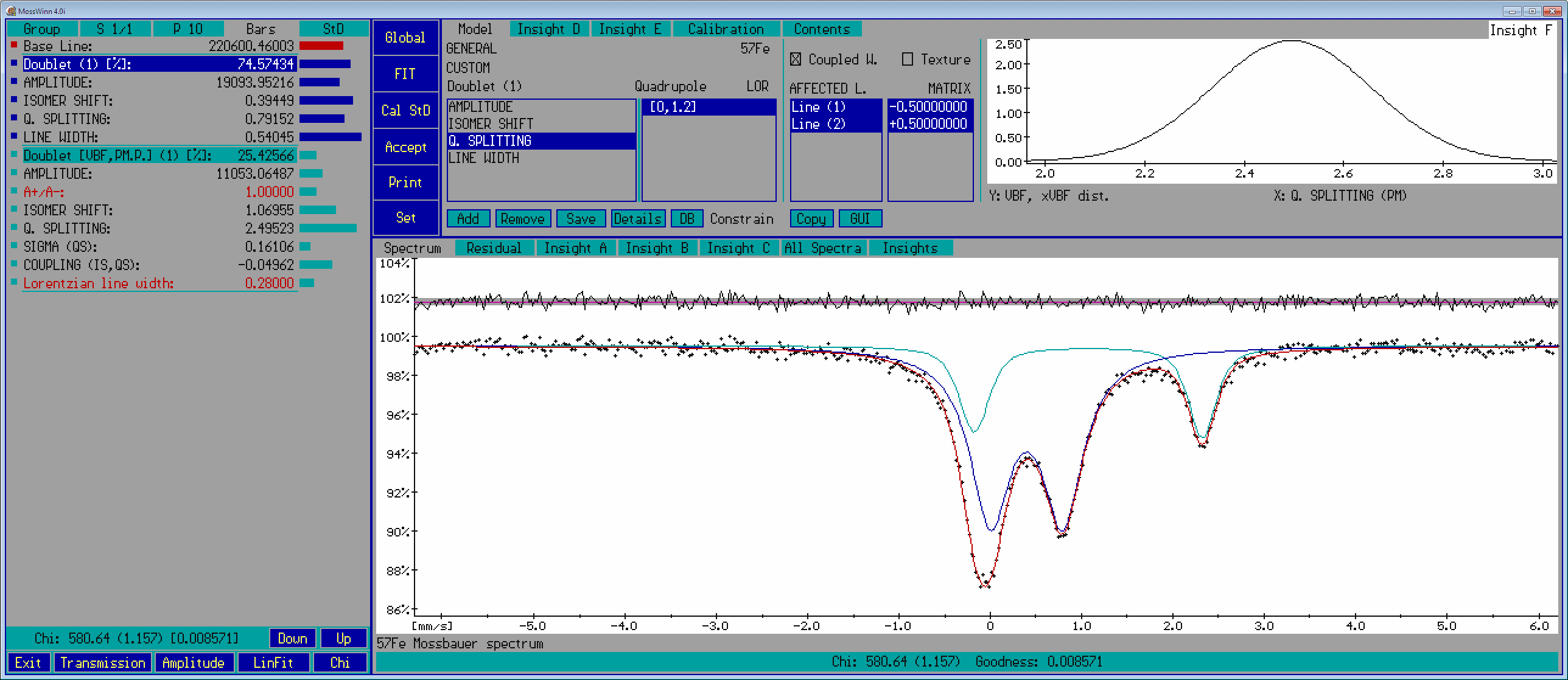
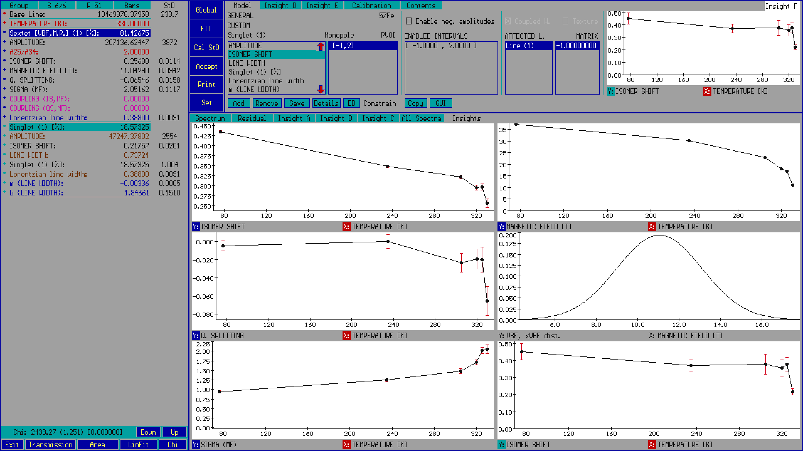
• The function of the menu boxes / visual elements - click on the menu box / visual element of interest.

• Parameter names and values - this panel shows the names and values of the fit parameters as well as the subspectrum headlines associated with the selected fit model, along with visual elements like the navigation / menu shapes (square or circle) before the parameter names, and the value-setting bars after the parameter values. In connection with the subspectrum headlines and the parameter names and values the following functionalities are available.

• Press on a parameter value with the left mouse button in order to edit the value in question. During editing characters can be selected by mouse, and selected (white) characters can be copied into the clipboard by pressing ctrl+C, as well as they can be pasted from the clipboard at the cursor position by pressing ctrl+V. In order to finish editing press enter or click with the mouse outside of the editing area. In order to cancel editing, press ESC.
 
• Press on the name of an unshared parameter with the left mouse button in order to fix / unfix the parameter in question. An unshared parameter is fixed if it is displayed with red color and it is free if it is displayed with darkgray color. The value of fixed parameters do not change during fitting.
• Press on the name of a shared parameter with the left mouse button in order to fix / unfix the parameter in question. A shared parameter can be fixed either independent of or together with the corresponding parameters in other - simultaneously fitted - spectra (example). Independently fixed shared parameters are displayed with red color. Shared parameters that are fixed to the same value in all the corresponding shared subspectra (sharefixed parameters - as we prefer to call them) are displayed by magenta color. A shared parameter is displayed with blue color if it is unfixed. The value of sharefixed parameters do not change during fitting.
• Press on the name of a parameter in a shared subspectrum with the right mouse button in order to share / unshare the parameter in question. A shared parameter can be unshared either by detaching it from the rest of the corresponding shared parameters (which latter will remain shared), or by setting the status of all the corresponding parameters to unshared / independent (example).

---

• A parameter is unshared if its value influences only the fit model set for the current spectrum.
• A parameter is shared if it is enforced to have the same value as the corresponding parameters in the models set for other spectra, and vice versa. A parameter can be defined to be shared only if simultaneous fitting of two or more spectra is performed. Only shared subspectra can have shared parameters.
• A subspectrum is shared if it exists in the model of two or more - simultaneously fitted - spectra. A fit model can include shared as well as unshared subspectra at the same time. The navigation / menu shapes of shared subspectra are circles (example). A shared subspectrum can be added to the fit model via the ADD menu box. The physical model associated with a shared subspectrum can only be changed coherently among the corresponding shared subspectra, i.e. if a shared subspectrum is modified in one of the simultaneously fitted spectra, then the modifications will take place in other simultaneously fitted spectra as well.
• A subspectrum is unshared if it is independent of the subspectra being part of models set for other - simultaneously fitted - spectra. Unshared subspectra cannot have shared parameters. The navigation / menu shapes of unshared subspectra are squares (example).

---

• Press on a subspectrum headline with the left mouse button in order to access the subspectrum's headline menu list with the following options.
• Rename subspectrum
• Add one more subspectrum of this type
• Unshare subspectrum in all of the spectra
• Unshare subspectrum in this spectrum only
• Delete subspectrum
• Fix all subspectrum parameters
• Unfix all subspectrum parameters
• Constrain parameters to be equal to those of
• Fit only this subspectrum
• Fit all but this subspectrum
• Copy peak positions and areas to clipboard / including information on nuclear states (example)

• Navigation / menu shapes (square or circle) help navigation among the parameters as they are displayed in the model page, as well as provide access to a popup menu with options concerning the corresponding subspectrum. Move the mouse pointer over the shape before a parameter in order to achieve the selection of the parameter on the model page. Press on one of the shapes in order to access the headline menu list of the corresponding subspectrum. The navigation / menu shapes of unshared subspectra are squares, while those of shared subspectra are circles. Parameters whose meaning/influence has been changed on the details page (with respect to their default meaning/influence for the given subspectrum type) are denoted by a menu shape with a light yellow center (example). Shared parameters for which the sharing constraint could not be satisfied for one or more of the simultaneously fitted spectra are denoted with a "strikethrough circle" (see below).

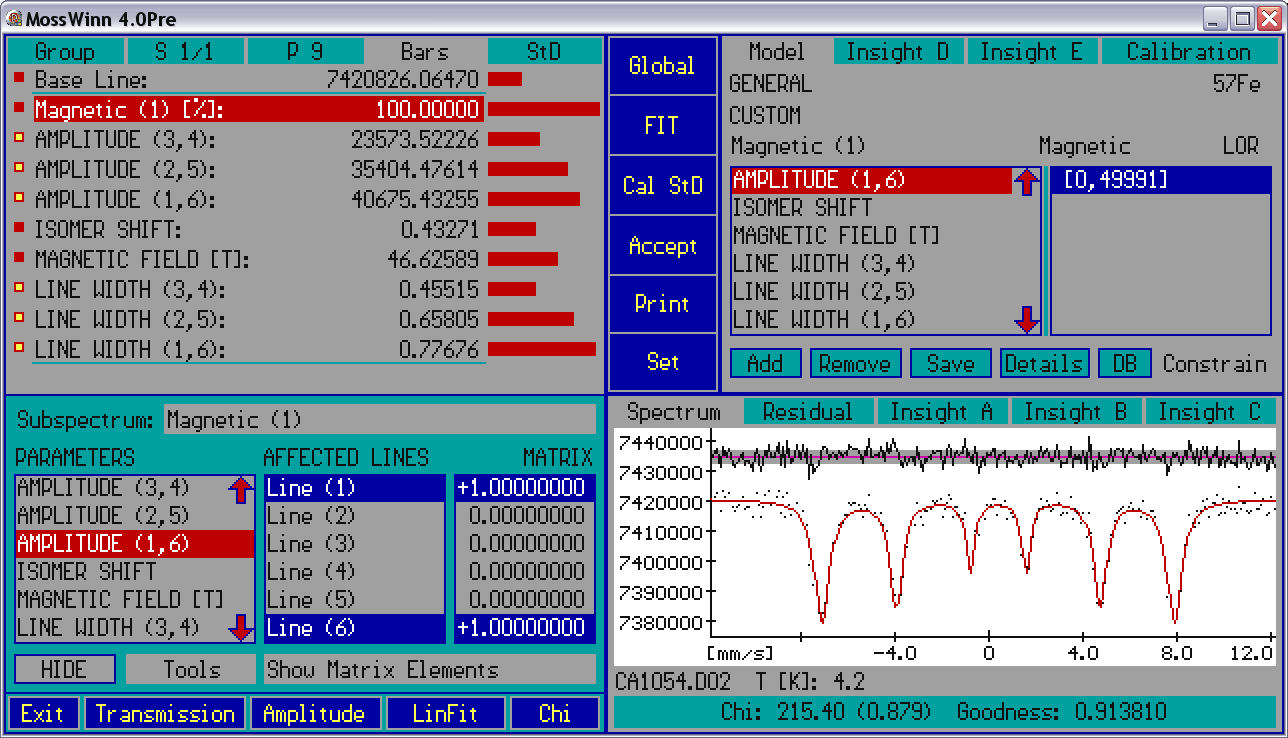
• - Parameter of an unshared subspectrum.
• - Parameter of an unshared subspectrum describing a linear model that was modified by the user such that the meaning of the parameter is unlike its default meaning. (The differences can be checked on the details page.)
• - Parameter of a shared subspectrum.
• - Parameter of a shared subspectrum describing a linear model that was modified by the user such that the meaning of the parameter is unlike its default meaning. (The differences can be checked on the details page.)
• - Parameter of a shared subspectrum for which a sharing constraint was set up, but for one or more of the simultaneously fitted spectra the sharing constraint could not be satisfied. (This may occur, e.g., for shared percentage parameters that may be subject to conflicting constraints in the different spectra.)

• Value-setting bars show the relative position of the corresponding parameter's current value between its allowed minimum and maximum values. If the current value of the parameter is lower than its minimum value, then the bar changes to a green arrow, whereas if it is higher than the allowed maximum value, then the bar changes to a red arrow (example). Press on the bar with the left mouse button in order to change the corresponding parameter value. In order to change the minimum or the maximum value allowed for a parameter, while pressing the left mouse button, move the mouse pointer outside the left- or right-side limit of the bar, and then press the right mouse button in addition to the left one.

• Down / Up - Press on these boxes in order to scroll the parameter list such that parameters below / above the lower / upper edge of the parameters' panel become visible and editable. Alternatively, the down / up arrow keys, the Page Down / Page Up keys, as well as the mouse wheel can also be used to achieve the same effect.

• The goodness of the (simultaneous) fit is emphasized in the bottom of the parameters' panel in the form of
  
  Chi: Chisquare (Normalized chisquare) [Goodness of fit]
  If the chosen theoretical model is correct, then an acceptable fit should provide a normalized chisquare close to 1, and a goodness of fit value higher than about 0.001 . In the case of simultaneous fitting of several spectra, these values characterize the simultaneous fit as a whole. In contrast, the corresponding values visible on the spectrum panel characterize only the fit of the current spectrum, as if it was the only one that is fitted. Accordingly, as long as only a single spectrum is fitted, the two panels show identical goodness-of-fit values.

• Group - Press on this menu box in order to change the apparent order of the subspectrum fit parameters (i.e. those following the parameter group of the base line) by selecting one of the following options.

• Group by Subspectra - Select this option in order to have fit parameters grouped first by subspectra and then by the type of parameters. Parameters belonging to the same subspectrum will follow each other in the following order: first the amplitude type parameters, then the position type parameters (which influence the position of the absorption peaks), then the width type parameters, and then the extra parameters if any. Each subspectrum parameter group is introduced by a headline showing the name and relative area fraction (in percentage) of the subspectrum, as well as a read-only bar whose length is proportional to the shown percentage value (example).
• Group by Parameter - Select this option in order to have fit parameters grouped first by the type of parameters and then by the subspectra they belong to. First the amplitude-, then the position-, then the width- and finally the extra type parameters — if any — will be displayed. Parameters of the same type will be grouped by subspectra (example).
• Group by Name - Select this option in order to have fit parameters grouped by the type of parameters and to have parameters of the same type ordered alphabetically. First the amplitude-, then the position-, then the width- and finally the extra type parameters — if any — will be displayed in alphabetical order (example).
• Show / Hide Subspectrum Name - Select this option in order to show / hide subspectrum headlines when fit parameters are grouped first by subspectra.

• S k/n indicates that the current spectrum is the kth from the n simultaneously fitted spectra. Press the TAB or the Backspace keys on the keyboard in order to navigate between the different simultaneously fitted spectra. If only a single spectrum is fitted, then S 1/1 is displayed. When simultaneous fitting of several spectra is performed, press on the corresponding box in order to access the following menu options in the appearing popup.

• Order spectra according to file name - select to order the fitted spectra alphabetically according to their file name.
• Order spectra according to parameter - select a fit parameter from the appearing list to have spectra ordered in an ascending manner with respect to the value of the selected parameter.
• Order spectra according to special parameter - select a special parameter from the appearing list to have spectra ordered in an ascending manner with respect to the value of the selected parameter.
• Reset original spectrum order - select this option to reset the original order of spectra that was set automatically when the FIT menu was entered.

The spectrum order set up via the above options will influence the order in which the spectra will follow each other when the TAB and Backspace keys are pressed, the order in which the spectra follow each other on the All Spectra tab, as well as the order in which spectra will appear on images printed to printer or copied to the clipboard.

• P n - indicates that the number of free parameters is equal to n. Free parameters are those which are actually adjusted / fitted when a fit procedure is initiated. Press on the corresponding box in order to access the following menu options in the appearing popup.

• Fix all parameters for the current spectrum - Select this option in order to achieve the following changes in the fix status of the fit parameters of the current spectrum:
• Free → Fixed
• Shared → Independently fixed shared
• Unfix all parameters for the current spectrum - Select this option in order to achieve the following changes in the fix status of the fit parameters of the current spectrum:
• Fixed → Free
• Independently fixed shared → Shared
• Independently fixed sharefixed → Sharefixed
• Reverse fix status of parameters for the current spectrum - Select this option in order to achieve the following changes in the fix status of the fit parameters of the current spectrum:
• Fixed ↔ Free
• Sharefixed ↔ Shared
• Independently fixed sharefixed ↔ Independently fixed shared
• Fix all parameters for all of the spectra - Select this option in order to achieve the following changes in the fix status of all the fit parameters:
• Free → Fixed
• Shared → Sharefixed
• Independently fixed shared → Independently fixed sharefixed
• Unfix all parameters for all of the spectra - Select this option in order to achieve the following changes in the fix status of all the fit parameters:
• Fixed → Free
• Sharefixed → Shared
• Independently fixed shared → Shared
• Independently fixed sharefixed → Shared
• Reverse fix status of parameters for all of the spectra - Select this option in order to achieve the following changes in the fix status of all the fit parameters:
• Fixed ↔ Free
• Sharefixed ↔ Shared
• Independently fixed sharefixed ↔ Independently fixed shared

(The fix status of nuclear and user-defined extra parameters — if any — will not be altered by selecting the above options.)

• Bars - Press on this tab in order to have the value-setting bars displayed on the right-hand side of the parameters' panel.

• StD - Press on this tab in order to follow the changes in the parameter values during fitting, or to display the standard deviation values of the parameters (example) after the StD values were calculated via a press on the Cal StD box. During fitting the displayed deviation values are calculated by subtracting the parameter's previous value from its new value, i.e. if the deviation is positive, then the parameter has increased in the last step of the fit. In order to change between the value-setting bars and the deviation values during fitting, position the mouse pointer over the parameters' panel, and then press space on the keyboard.

• Chi - Press on this box in order to access the following options related to the fitness function and the corresponding calculation of the goodness-of-fit parameter.

• Weighted squared deviation (Chisquare) - Select this option to have chisquare minimized during fitting.
• Simple squared deviation - Select this option to have the sum of simple squared deviations - between the measured and calculated data points - minimized during fitting.
• Absolute deviation - Select this option to have the sum of absolute deviations - between the measured and calculated data points - minimized during fitting.
• Do not ignore zero points for current spectrum - Select this option in order to have zero-valued data points of the current spectrum considered during fitting.
• Ignore zero points for all fitted spectra - Select this option in order to have zero-valued data points ignored in all the fitted spectra. Ignored data points are not taken into account when the goodness of the fit is calculated, consequently they do not influence the results of the fit.

• LinFit - Press on the LinFit box with the left mouse button in order to optimize the Base Line and Amplitude type parameters of the model set for the current spectrum in a single step. Press on it with the right mouse button in order to do the same optimization for all the simultaneously fitted spectra. The value of position-, width- and extra type parameters will not be altered.

• Amplitude / Area - Press on this box in order to toggle between Amplitude and Area modes of the calculation of individual absorption peaks. This setting influences all the simultaneously fitted spectra. When area mode is selected then amplitude type parameters are treated as area type parameters, i.e. they are assumed to determine the area under individual peaks. If amplitude mode is selected, then the amplitude-type parameters determine the amplitude of the individual peaks. At the same time, even if area / amplitude mode is selected, amplitude-type parameters are not necessarily equal to the area / amplitude of the associated peaks, because the factors connecting the peak parameters to the amplitude-type fit parameters may also influence the calculated peak areas / amplitudes. (These factors can be set on the Details page). Independent of whether Amplitude or Area mode is set, for theoretical models that cannot be altered by such factors (e.g. Hamiltonian models), the amplitude-type parameter always denotes the area under the whole subspectrum. The area under the individual subspectra can also be calculated on the basis of the Total Spectrum Area (TSA) and the relative subspectrum areas displayed on the fit report for each of the subspectra being part of the fitted model.

• Transmission / Reflection - Press on this box in order to toggle between transmission and reflection geometry modes for the current spectrum. Transmission refers to transmission Mossbauer spectroscopy where peaks are subtracted from the background, whereas Reflection refers to scattering geometries like CEMS or XMS where the peaks are added to the background.

• Exit - Press on this box with the left mouse button to leave the FIT menu and have distribution curves — if any — appearing in the main menu as separate windows. Press on it with the right mouse button in order to leave the fit menu without having distribution curves to appear in the main menu. Note that fit results are not automatically saved to the fitted spectra - press on the Accept box in order to achieve that.

• Global - Press on the Global menu box in order to initiate global fitting of model parameters. The global fitting procedure is based on a robust numerical optimization method realized by a special evolution algorithm developed especially for the purposes of Mossbauer spectrum analysis. (See NIM B 129 (1997) 527 for details.) Global fitting is able to locate the global optimum of the set of fitting parameters even if the initial parameter set is very far from being optimal. Global fitting fully respects the allowed parameter ranges, i.e. it will never produce a result that is outside of these ranges. (Consequently, if the optimum solution is outside of the preset ranges, then the global fitting procedure cannot succeed.) Global fitting is infinite: press the ESC key on the keyboard in order to terminate the fit. After global fitting was stopped, one usually turns to the FIT menu box in order to finish up the fit by local tuning of the fit parameters.

• FIT - Press on the FIT menu box with the left mouse button in order to initiate local tuning of the fit parameters starting from the current parameter set. Local tuning does not respect the constraints imposed on the allowed parameter ranges, unless the constraints in question are designated to be HARD. Local tuning stops automatically after it has been converged with high precision. However, if lower precision is also acceptable one can also stop the fit manually by pressing the ESC key on the keyboard. Whether manual stopping resulted in an acceptable solution can be verified by calculating the standard deviation of the parameters via the Cal StD menu box: if the standard deviation values can be calculated without MossWinn reporting about an error, then the manual stopping of the fit procedure was valid. Press on the FIT menu box with the right mouse button in order to access one of the following options.

• Fit using METHOD A - Initiates local tuning of the fit parameters by using Method A (equivalent to the left mouse click on the FIT menu box).
• Fit using METHOD B - Initiates local tuning of the fit parameters by using Method B that is more robust but - on average - converges slower than Method A.
• Linear Fit Amplitudes - Select this option to optimize the Base Line and Amplitude type parameters of the model set for the current spectrum in a single step (eqivalent to the effect of a left mouse click on the LinFit box).
• Fit current spectrum only - Select this option in order to adjust only those fit parameters that are part of the model set for the current spectrum. It is the simultaneous goodness of fit that is optimized, such that in the case of simultaneous fitting of multiple spectra - and in the presence of shared parameters - the final result may also be influenced by the other spectra fitted.
• Fit spectra sequentially - Select this option in order to carry out the previous function (Fit current spectrum only) for all the simultaneously fitted spectra one after the other. After the last spectrum was also fitted in this way, the fit starts again with the first one, and so on until convergency is achieved.
• Fit only Amplitudes - Select this option in order to fit only the base line and the amplitude-type parameters for all the simultaneously fitted spectra.
• Fit only Positions - Select this option in order to fit only the position-type parameters for all the simultaneously fitted spectra.
• Fit only Line Widths - Select this option in order to fit only the width-type parameters for all the simultaneously fitted spectra.
• Fit only Extra Parameters - Select this option in order to fit only the extra-type parameters (i.e. those which follow the width-type parameters) for all the simultaneously fitted spectra.

• Cal StD - Press on the Cal StD menu box with the left mouse button in order to calculate the standard deviation of the fitting parameters by assuming that they represent the result of a convergent fit. The calculations are based on the approximation of the curvature matrix (one-half times the Hessian matrix) of the chisquare quantity. The method used for the calculation of the chisquare quantity depends on the fitness function optimized during the fit. The calculations can proceed via the numerical approximation of either the 1st derivatives of the fit model envelope or the 2nd derivatives of the chisquare quantity with respect to the fit parameters. Turn to the Configuration settings... option of the SET menu, in order to determine which of the two methods gets invoked by pressing on the Cal StD menu box.
  
  Press on the Cal StD menu box with the right mouse button in order to access one of the following options.

• Copy correlation matrix to clipboard - Turn to this option in order to copy the correlation matrix of fit parameters into the Windows clipboard. Element (i,j) of the correlation matrix is calculated as COV(i,j)/[COV(i,i)COV(j,j)]^½ where COV(i,j) denotes element (i,j) of the covariance matrix, the latter being equal to the inverse of the curvature matrix of chisquare. The correlation matrix becomes recalculated each time the StD of parameters is calculated via the inversion of the curvature matrix. As the output format of the correlation matrix the following options are available.
• As image (for all spectra) - The correlation matrix will be copied into the clipboard as a grayscale bitmap image. All the fitted spectra are considered. The cells of the matrix image are shaded according to the corresponding correlation value: higher correlation values are denoted by a darker shade of gray. Spectra, subspectra and parameters are shaded as their darkest-shaded subspectrum, parameter and correlation value, respectively (example). Invalid values (either referring to a fit that is not optimal, or signalling the occurrence of a singularity during matrix inversion) are denoted by a question mark on a black background.
• As image (for current spectrum) - The correlation matrix will be copied into the clipboard as a grayscale bitmap image. Only those fit parameters are considered, that belong to the fit model of the current spectrum.
• As image (value limited, for all spectra) - The correlation matrix will be copied into the clipboard as a grayscale bitmap image. Only those fit parameters are considered that display correlation values higher than or equal to the value set by the user. This option is especially useful to reduce the size of the correlation matrix - and restrict it to the potentially most problematic parameters - by excluding parameters that do not display appreciable correlation.
• As text (for all spectra) - The correlation matrix will be copied into the clipboard as a table given as comma delimited text. All the fitted spectra are considered.
• As text (for current spectrum) - The correlation matrix will be copied into the clipboard as a table given as comma delimited text. Only those fit parameters are considered, that belong to the fit model of the current spectrum.
• As text (value limited, for all spectra) - The correlation matrix will be copied into the clipboard as a table given as comma delimited text. Only those fit parameters are considered that display correlation values higher than or equal to the value set by the user. This option is especially useful to reduce the size of the correlation matrix - and restrict it to the potentially most problematic parameters - by excluding parameters that do not display appreciable correlation.
• Save correlation matrix - Turn to this option in order to save the correlation matrix of fit parameters as a GIF image file that is optimal for being inspected by the help of web browsers. As the output format of the correlation matrix the following options are available.
• As GIF image (for all spectra) - The GIF image of the correlation matrix is saved by considering all the fitted spectra.
• As GIF image (for current spectrum) - The GIF image of the correlation matrix is saved by considering only those fit parameters that belong to the fit model of the current spectrum.
• As GIF image (value limited, for all spectra) - The GIF image of the correlation matrix is saved by considering only those fit parameters that display correlation values higher than or equal to the value set by the user.
• Approximate StD via 1st derivatives - Select this option in order to calculate the standard deviation of the fit parameters via the approximation of the curvature matrix on the basis of the numerical approximation of the 1st derivatives of the fit model envelope with respect to the fit parameters, by assuming that the current set of fit parameters represents the result of a convergent fit. This method is in general faster and more reliable — especially in cases involving the fit of hyperfine parameter distributions — than the method based on the approximation of the chisquare 2nd derivatives.
• Approximate StD via 2nd derivatives - Select this option in order to calculate the standard deviation of the fit parameters via the approximation of the curvature matrix on the basis of the numerical approximation of the 2nd derivatives of the chisquare quantity with respect to the fit parameters, by assuming that the current set of fit parameters represents the result of a convergent fit. This method is susceptible to failure when the fit involves hyperfine parameter distributions, in which case the method based on the approximation of the 1st derivatives could be used to observe the StD values of fit parameters.
• Approximate StD via Monte Carlo iterations - Select this option in order to calculate the standard deviation of the fit parameters via Monte Carlo iterations by assuming that the current set of fit parameters represents the result of a convergent fit. This method is more robust but works slower than the default method based on the approximation of the curvature matrix. Assuming that the fitting envelop represents well the measured data, and that the measured counts distribute around their expected values normally, the program generates hypothetical spectra (that could have been observed in repeated measurements) and fits the theoretical model to all of them one after the other. (When the fitness function is the chisquare the variance of the counts is assumed to be equal to the value of the counts in accordance with the underlying Poisson statistics, whereas when the fitness function is the Simple squared deviation or the Absolute deviation, a uniform variance is assumed and estimated on the basis of the counts and the fit model curve.) The standard deviation of the model parameters is then estimated on the basis of the statistics of the parameter values obtained in the subsequent fits. 100 iterations usually provide sufficient precision in practice. By the use of this method one can also estimate the reliability of distribution data points: the program records the value of every distribution data point during the subsequent iterations, and on the distribution graph it draws the minimum and the maximum for each data point by blue and red color, respectively. On the basis of the figure observed (example) in this way one can have an impression of how reliable the observed distribution is.
• Clear StD values - Select this option in order to clear the calculated standard deviation values of the fit parameters.
• Approximate reliability of distributions - Based on the principle of Monte Carlo iterations detailed above, this option provides a faster alternative for the estimation of the reliability of distributions. In the case of the present option the fit parameters are kept fixed to their original values, and the fit of the hypothetical spectra is optimized only by recalculating the distribution curve. Although this method can be expected to show distribution curves to be more reliable than they actually are, in practice it is a rather useful method especially to rule out unreliable distribution curves.
• Reset distribution graphs - Turn to this option in order to remove the blue (minimum) and red (maximum) curves - calculated by the above mentioned Monte Carlo error estimation procedures - from the distribution graphs (if any).

• Accept - Press on the Accept menu box with the left mouse button in order to save the current status of the fit to the data file associated with the fitted spectrum. The fit result accepted in this way becomes automatically reloaded when next time the FIT menu is entered for the same spectrum. Accepting a fit result will overwrite any fit result accepted previously for the same spectrum file. In the case of simultaneous fitting of several spectra, the complete status of the fit is saved, and the simultaneous fit is recovered when next time the fit menu is entered for any of the spectra for which the corresponding simultaneous fit result was accepted. (To accomplish this recovery task, MossWinn may need to load in spectra if required by the saved simultaneous fit, which is then carried out automatically while the FIT menu is being entered.) Normally, after a successful fit was carried out, it is recommended to accept the fit. (Note that the TBL menu creates tables of fit parameters on the basis of accepted fit results.) When the option of Automatic HTML FitLog creation on Accept is enabled via the performance settings, then the current status of the fit is furthermore also saved (cumulatively, but without duplicates) to the respective HTML FitLog files of the fitted spectra. In order to access further functions related to the accepted / logged fit statuses, press on the Accept menu box with the right mouse button, and select one of the following options.

• Revert to previously accepted fit parameter values - Select this option in order to reload the value of those actually defined fit parameters that were also included in the fit accepted previously for the current spectrum (via an LMC on the Accept menu box). (The fit model itself is not reloaded, i.e. the number and kind of the subspectra — contributing to the actually set fit model — will not be altered.)
• Save HTML FitLog according to the present state - Select this option in order to save a HTML FitLog to the FitLog file of the current spectrum, according to the current state of the fit.
• Reload previously logged fit model... - Select one of the submenus of this menu option in order to reload and set the corresponding fit model from the FitLog file associated with the current spectrum. The currently set fit model will be overwritten.
• Delete FitLog from log file... - Select one of the submenus of this menu option in order to remove the corresponding FitLog from the FitLog file associated with the current spectrum.
• Delete all FitLogs but the last / for all the fitted spectra - Select this menu option in order to remove all but the last saved FitLog from the FitLog file associated with the current spectrum. Select the appearing submenu item in order to carry out the same operation for all the simultaneously fitted spectra.

• Print - Press on the Print menu box with the left mouse button in order to carry out the default print operation assigned to the Print menu box in the corresponding submenu of the SET menu box. Press on the Print menu box with the right mouse button in order to access one of the following options.

• Print fit results as text - Select this option in order to print the textual fit report associated with one or more of the fitted spectra to the default printer (example). In order to send the print job to a different printer, select the printer in question from the appearing list.
• Print current spectrum - Select this option in order to print the graph of the current spectrum to the printer set as default in the SET menu. In order to send the print job to a different printer, select the printer in question from the appearing list.
• Print current spectrum + distributions - Select this option in order to print the graph of the current spectrum and those of the fitted distributions (if any) to the printer set as default in the SET menu. The graphs are all printed on the same page. In order to send the print job to a different printer, select the printer in question from the appearing list.
• Print fit results + spectrum + distributions - Select this option in order to print to the default printer the textual fit report(s), and then on separate page (pages) the graph (graphs) of the spectrum (spectra) and fitted distributions (if any). In order to send the print job to a different printer, select the printer in question from the appearing list.
• Print all spectra - Select this option in order to print to the default printer the graph of all the simultaneously fitted spectra, on a single page. In order to send the print job to a different printer, select the printer in question from the appearing list.

---

• Copy to clipboard as text - Select this option in order to copy the textual fit report associated with the current spectrum to the clipboard of Windows (example).
• Copy all to clipboard as text - Select this option in order to copy the textual fit report of all the simultaneously fitted spectra to the clipboard of Windows. If a parameter (submenu item) is selected, then the individual fit reports will follow each other in order according to the value of the selected parameter.
• Copy to clipboard as table for graphics - Select this option in order to copy the fit results to the clipboard as comma-delimited text forming a table in which the parameters characterizing a particular spectrum are all listed in a single row, whereas each parameter - as well as each standard deviation value - has its own column (example). This arrangement is especially useful for drawing the value of some parameter (e.g. isomer shift) as a function of another one (e.g. temperature) by the help of an external grapher program.
• Copy to clipboard as table for presentation - Select this option in order to copy the fit results to the clipboard as comma-delimited text forming a table in which the parameters characterizing a particular spectrum are all listed in a single column, whereas each parameter has its own row (example). This arrangement is considered to be useful when creating tables for a presentation.
• Copy current spectrum to clipboard - Select this option in order to copy the graph of the current spectrum to the clipboard of Windows according to the default settings attributed to Clipboard - single spectrum on the Printer Setup Dialog.
• Copy current spectrum + distributions to clipboard - Select this option in order to copy the graph of the current spectrum and those of the fitted distributions (if any) to the clipboard of Windows.
• Copy all Insight Pages to clipboard - Select this option in order to copy the graphical content of non-empty insight pages (if any) to the clipboard of Windows.
• Copy all spectra to clipboard - Select this option in order to copy the graph of all the simultaneously fitted spectra to the clipboard of Windows (example). If a parameter (submenu item) is selected, then the spectrum graphs will be arranged according to the value of the selected parameter.

---

• Save and open as HTML FitLog - Select this option in order to save and open a HTML FitLog for one or more of the fitted spectra according to the current state of the fit. The FitLog file is saved to the folder that contains also the corresponding spectrum data file, and it is opened in the default web browser application.

---

• Save as simple text - Select this option in order to save the fit report of the current spectrum as text file (example).
• Save all as simple text - Select this option in order to save the fit report of all the simultaneously fitted spectra in the same text file one after the other.
• Save as table for graphics - Select this option in order to save the fit results as comma-delimited text into a text file forming a table in which the parameters characterizing a particular spectrum are all listed in a single row, whereas each parameter - as well as each standard deviation value - has its own column (example). This arrangement is especially useful for drawing the value of some parameter (e.g. isomer shift) as a function of another one (e.g. temperature) by the help of an external grapher program.
• Save as table for presentation - Select this option in order to save the fit results as comma-delimited text into a text file forming a table in which the parameters characterizing a particular spectrum are all listed in a single column, whereas each parameter has its own row (example). This arrangement is considered to be useful when creating tables for a presentation.

• Set - Press on the Set menu box in order to access one of the following options.

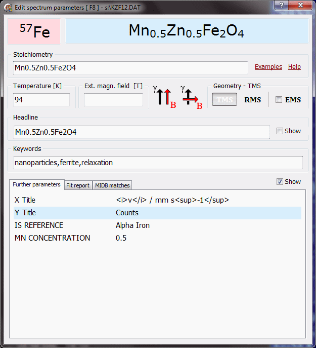
• Spectrum parameters - Turn to this option in order to set/modify spectrum parameters associated with the current spectrum.
• Isomer shift reference - Turn to this option in order to set/modify the isomer shift of the isomer shift reference material (associated with the current source nuclide) relative to the corresponding standard IS reference material. The value given here is considered when the fitness of MIDB records is evaluated (with respect to the current spectrum) for example when the Find and apply best match submenu option of the DB menu is selected.
• Line widths... - Turn to this option in order to constrain all line width type parameters of the current model to have always the same value, or to make all line width type parameters independent. To impose more refined constraints of this type, turn to the Constrain menu.
• Constrain all to be same
• Set all to be independent
• Parameter boundaries... - Turn to this menu to access the following options.
• Share for the selected parameter (The constraints imposed on the selected parameter will be set for the corresponding parameters in the simultaneously fitted spectra.)
• Share for position and width parameters (The constraints imposed on the position and width type parameters of the selected subspectrum will be set for the corresponding parameters in the simultaneously fitted spectra.)
• Share for all position and width parameters (The constraints imposed on the position and width type parameters of the current spectrum will be set for the corresponding parameters in the simultaneously fitted spectra.)
• Stretch to make current parameter values valid (For parameters whose value lies outside of the allowed range, the parameter boundaries will be extended such that the allowed range includes the current value of the parameter.)
• If Lorentzian with dispersion is selected as line shape... - Turn to this option in order to enable / disable mixing of the Lorentzian with dispersion line shape with other type of line shapes in the same model. Normally, in the case of interference with the atomic photoelectric effect (see PRL 28 (1972) 530 and PRC 8 (1973) 1916), it is physically reasonable to fit all the absorption peaks with the Lorentzian with dispersion line shape.
• Set it only for the selected subspectrum
• Set it for all the subspectra
• Enable / Disable subspectrum calculation for Transmission Integral - Normally, if transmission integral is used to fit a spectrum with more than one subcomponents, then subspectrum curves are formally indicated emphasizing the corresponding nuclear absorption spectrum. (In such a case, however, the fitting curve cannot be produced by the simple addition of the indicated subspectra.) Select this option in order to enable / disable the calculation of such subspectra.
• Determine parameter values with a relative precision of - Turn to this option in order to determine the relative precision by which the fit parameters associated with a local optimum should be determined during the fit procedure.
• Enable negative amplitude/area values / Force non-negative amplitude/area values - Turn to these options in order to determine whether amplitude type parameters can take on negative values or not. Normally, amplitude type parameters should be forced to be non-negative.
• Enable negative line width values / Force positive line width values - Turn to these options in order to determine whether line width type parameters can take on negative values or not. Normally, line width type parameters should be forced to be positive. (Setting of negative line width values may lead to meaningless results.)
• Remove calibration of the current spectrum - Select this option in order to erase the calibration of the velocity axis, i.e. to make the horizontal axis to display channel numbers instead of velocity values.
• Set GUI resolution... - Select this option to set the internal resolution of the graphical user interface (GUI).
• Configuration settings... - Select this option to set various configuration parameters influencing the operation of MossWinn.
• Left mouse click on the Print box should... - Turn to this menu in order to determine what should happen when the Print box is pressed on by the left mouse button.
• Print fit results as text
• Print fit results and then the spectrum
• Print fit results then the spectrum + distributions
• Copy fit results to the clipboard

• Model - click on the Model tab in order to access the model page that allows the setting of the attributes of the fit model set for the current spectrum. The function of the various visual elements of the model page are listed below.

• Model groups popup box (GENERAL) - Press on this area with the left mouse button in order to access the model groups and the corresponding fit models that were saved earlier via the Save Model As menu. One can select here either a model group or directly one of the fit models. When multiple spectra are fitted simultaneously, the selected model can be set either for the current spectrum or for all the simultaneously fitted spectra at once. Originally only a single model group, named GENERAL, is defined. Each model group can contain around 32 fit models, and there can be around 32 model groups allowing to manage more than 1000 fit models altogether.
• Models popup box (CUSTOM) - Press on this area with the left mouse button in order to access the models (saved earlier via the Save Model As menu) of the currently selected model group. When multiple spectra are fitted simultaneously, the selected model can be set either for the current spectrum or for all the simultaneously fitted spectra at once. Originally each model group contains only a single model, named CUSTOM. The CUSTOM model of a model group contains the fit model that was abandoned when the model group in question was selected.
• Source popup box (57Fe) - Press on the source popup box to select the Mossbauer nuclide / transition that was used to measure the fitted spectra. The same nuclide / transition is set for all the simultaneously fitted spectra. If one of the transition types (M1/E1, M1+E2, E2) is selected then the nuclear parameters (nuclear spin, g-factor, quadrupole moment, etc.) are added to the parameter list of the background as fixed parameters. When unfixed, the nuclear parameters can be fitted as well.
• Subspectrum popup box - Press on the subspectrum popup box in order to select one of the subspectra being part of the fit model set for the current spectrum. The parameters of the selected subspectrum will appear in the parameter list box. The parameter list of the spectrum background is formally treated here as the 0th subspectrum named Background.
• Parameter list box - This list box displays the parameters belonging to the subspectrum currently selected in the Subspectrum popup box. Press on the name of one of the parameters in order to make the corresponding parameter constraints become listed in the parameter constraints list box on the right. Press on the arrows or use the mouse wheel in order to scroll the list of parameters up or down. A parameter can also be selected by moving the mouse pointer over the corresponding navigation shape on the parameters panel.
• Parameter constraints list box - This list box displays the constraints imposed on the parameter currently selected in the parameter list box. Some of the constraints can be edited manually: press on such constraints with the left mouse button in order to edit them. In order to delete a constraint, erase all of its characters in edit mode. Press on a constraint with the right mouse button in order to disable / enable it, without deletion. A constraint is in effect (i.e. enabled) only if it is written with white color on a blue background. One cannot delete or disable all of the constraints: at least one of them has to remain in effect. Whereas parameter constraints are always obeyed by the Global Fit procedure, the local fit procedure respects only those constraints that are marked to be a Hard constraint by the help of the corresponding menu of the Constrain popup box. If for a parameter more than one constraint is defined, then the enabled constraints are evaluated from top to bottom one after the other. The result of the evaluation (i.e. the ranges enabled for the parameter) can be examined on the Details page. In the following examples of constraints are listed together with their meaning.

• [0.1,1.2] - the parameter has to remain in the range of 0.1 – 1.2 .
• [-3.4] - the parameter has to be equal to -3.4.
• INC [45,55] - the parameter can take on values in the range of 45 – 55 .
• EXC [50,52] - the parameter cannot take on values of the range 50 – 52 .
• > 1.5 - the parameter should be higher than 1.5 .
• <= 2.1 - the parameter should be less or equal 2.1 .
• HARD - the parameter constraints should be obeyed also by the local fit procedure.
• [0.2,1.2]
  EXC [0.5,1]
  INC [0,0.1]
  INC [0.6,0.7] - If all the four of the above constraints are defined in this order for a single parameter, then the parameter in question can take on values only in the range of [0,0.1] ∪ [0.2,0.5) ∪ [0.6,0.7] ∪ (1,1.2].

• Interaction popup box - Press on this popup box in order to select the — built-in or user-written external (DLL) — theoretical model to be applied to the current subspectrum. Built in theoretical models available, e.g., for ⁵⁷Fe are listed below.

• Monopole - a single absorption peak (singlet).
• Quadrupole (Powder) - quadrupole doublet consisting of two peaks of equal amplitudes and line widths. Linear model, it can be altered on the Details page.
• Magnetic (Powder) - magnetic sextet consisting of six peaks having equal line widths and relative amplitudes of 3:2:1:1:2:3. Linear model, it can be altered on the Details page.
• First Order Mixed M+Q (Powder) - magnetic sextet consisting of six peaks having equal line widths and relative amplitudes of 3:2:1:1:2:3. The sextet takes quadrupole interaction into account by treating the quadrupole interaction as a small perturbation of the magnetic one: the two outermost lines of the sextet are shifted along the velocity axis by +Δ/2 whereas the four inner lines are shifted by -Δ/2, where Δ is the quadrupole splitting. Linear model, it can be altered on the Details page.
• Mixed M+Q Static Hamiltonian (Powder) - in general 8 peaks with equal line width, having positions and amplitudes calculated by solving the static Hamiltonian of mixed magnetic and quadrupole interactions. The e_z basis vector of the reference coordinate system (figure) is assumed to be parallel to the hyperfine magnetic field.
• Mixed Q+M Static Hamiltonian (Powder) - in general 8 peaks with equal line width, having positions and amplitudes calculated by solving the static Hamiltonian of mixed magnetic and quadrupole interactions (as described in NIM 48 (1967) 219). The e_z basis vector of the reference coordinate system (figure) is assumed to be parallel to the z axis of the eigensystem of the EFG.
• Blume-Tjon Two State Magnetic Relaxation (Powder) - model of uniaxial superparamagnetic relaxation as described in PR 165 (1968) 446.
• Tjon-Blume Jahn-Teller Quadrupole Relaxation (Powder) - model considering quadrupole interaction in the presence of a fluctuating electric field gradient, expected e.g. in the case of the dynamic Jahn-Teller effect. Described in PR 165 (1968) 456.
• Electron Hopping Relaxation (Paramagnetic, Powder) - model implemented for ⁵⁷Fe in paramagnetic powder where electron hopping occurs either between iron ions of different oxidation states (e.g. Fe²⁺ ↔ Fe³⁺) or between iron ions and the rest of the system. It can model situations encountered, e.g., in Phys. Chem. Minerals 10 (1984) 250. and PRB 31 (1985) 34.
• Electron Hopping Relaxation (Magnetic, Powder) - model implemented for ⁵⁷Fe in a magnetic powder where electron hopping occurs either between iron ions of different oxidation states (e.g. Fe²⁺ ↔ Fe³⁺) or between iron ions and the rest of the system. It can model situations encountered, e.g., in J. Phys. Chem. Solids 41 (1980) 1273.
• Random EFG in uniaxial external magnetic field (Powder) - model of a powdered sample with randomly oriented EFG (displaying zero asymmetry parameter) and uniaxial hyperfine magnetic field, as described in NIM B 9 (1985) 201.


• Paramagnetic Hyperfine Structure (Powder)... - paramagnetic hyperfine structure models, as listed below. These models require either the DBM version of MossWinn or subscription to the MossWinn services. See examples and the manual for further details.
• PHS 1/2 (Powder, ZERO EMF, Slow R.) - accounts for a powder sample with an electronic system with effective spin S = ½, by assuming slow electronic relaxation in the absence of an external magnetic field. The eigensystem of the hyperfine magnetic interaction tensor (A) and the electric field gradient tensor (EFG) are assumed to be coincident. See, for example, Phys. Rev.152 (1966) 345.
• PHS (Powder, ZERO EMF, Slow R.) - accounts for a powder sample with an electronic system with effective spin S = 0...5/2, by assuming slow electronic relaxation in the absence of an external magnetic field. The eigensystem of the hyperfine magnetic interaction tensor (A) and the electric field gradient tensor (EFG) are assumed to be coincident with the x,y,z crystal field system (CFS). See, for example, Rep. Prog. Phys. 16 (1953) 108-159. and Phys. Rev. 148 (1966) 211.
• PHS Trigonal (Powder, ZERO EMF, Slow R.) - accounts for a powder sample with an electronic system with effective spin S = 0...5/2, by assuming slow electronic relaxation in the absence of an external magnetic field. The eigensystem of the hyperfine magnetic interaction tensor (A) and the electric field gradient tensor (EFG) are assumed to be coincident with the x,y,z crystal field system (CFS) whose z axis is oriented in the (1,1,1) cube diagonal direction of the cubic crystal field system (trigonal distortion). Tensor A is assumed to display axial symmetry (A_yy = A_xx). See, for example, Biochemistry (Structure and Bonding) 20 (1974) 59..
• PHS Angle (Powder, ZERO EMF, Slow R.) - accounts for a powder sample with an electronic system with effective spin S = 0...5/2, by assuming slow electronic relaxation in the absence of an external magnetic field. The eigensystem of the hyperfine magnetic interaction tensor (A) and the electric field gradient tensor (EFG) are given with respect to the x,y,z crystal field system (CFS) via the respective Euler angles that rotate the CFS system into the A or EFG tensor eigensystem. The orientation of the x,y,z CFS system is given with respect to the [100, 010, 001] cubic system via the Euler angles that rotate the cubic system into the CFS system.


• PHS 1/2 (Powder, EMF, Slow R.) - accounts for a powder sample with an electronic system with effective spin S = ½, by assuming slow electronic relaxation in an external magnetic field oriented either parallel or perpendicular to the Mössbauer γ-ray direction. The eigensystem of the electron gyromagnetic tensor (g), the hyperfine magnetic interaction tensor (A) and the electric field gradient tensor (EFG) are assumed to be coincident.
• PHS (Powder, EMF, Slow R.) - accounts for a powder sample with an electronic system with effective spin S = 0...5/2, by assuming slow electronic relaxation in an external magnetic field oriented either parallel or perpendicular to the Mössbauer γ-ray direction. The eigensystem of the electron gyromagnetic tensor (g), the hyperfine magnetic interaction tensor (A) and the electric field gradient tensor (EFG) are assumed to be coincident with the x,y,z crystal field system (CFS).
• PHS Trigonal (Powder, EMF, Slow R.) - accounts for a powder sample with an electronic system with effective spin S = 0...5/2, by assuming slow electronic relaxation in an external magnetic field oriented either parallel or perpendicular to the Mössbauer γ-ray direction. The eigensystem of the electron gyromagnetic tensor (g), the hyperfine magnetic interaction tensor (A) and the electric field gradient tensor (EFG) are assumed to be coincident with the x,y,z crystal field system (CFS) whose z axis is oriented in the (1,1,1) cube diagonal direction of the cubic crystal field system (trigonal distortion). Tensors g and A are assumed to display axial symmetry (g_yy = g_xx, A_yy = A_xx).
• PHS Angle (Powder, EMF, Slow R.) - accounts for a powder sample with an electronic system with effective spin S = 0...5/2, by assuming slow electronic relaxation in an external magnetic field oriented either parallel or perpendicular to the Mössbauer γ-ray direction. The eigensystem of the electron gyromagnetic tensor (g), the hyperfine magnetic interaction tensor (A) and the electric field gradient tensor (EFG) are given with respect to the x,y,z crystal field system (CFS) via the respective Euler angles that rotate the CFS system into the g, A or EFG tensor eigensystem. The orientation of the x,y,z CFS system is given with respect to the [100, 010, 001] cubic system via the Euler angles that rotate the cubic system into the CFS system.


• PHS 1/2 (Powder, EMF, Decoupled, Fast R.) - accounts for a powder sample with an electronic system with effective spin S = ½ being decoupled from the nuclear spin states, by assuming fast electronic relaxation in an external magnetic field oriented either parallel or perpendicular to the Mössbauer γ-ray direction. The eigensystem of the electron gyromagnetic tensor (g), the hyperfine magnetic interaction tensor (A) and the electric field gradient tensor (EFG) are assumed to be coincident.
• PHS (Powder, EMF, Decoupled, Fast R.) - accounts for a powder sample with an electronic system with effective spin S = 0...5/2 being decoupled from the nuclear spin states, by assuming fast electronic relaxation in an external magnetic field oriented either parallel or perpendicular to the Mössbauer γ-ray direction. The eigensystem of the electron gyromagnetic tensor (g), the hyperfine magnetic interaction tensor (A) and the electric field gradient tensor (EFG) are assumed to be coincident with the x,y,z crystal field system (CFS).
• PHS Trigonal (Powder, EMF, Decoupled, Fast R.) - accounts for a powder sample with an electronic system with effective spin S = 0...5/2 being decoupled from the nuclear spin states, by assuming fast electronic relaxation in an external magnetic field oriented either parallel or perpendicular to the Mössbauer γ-ray direction. The eigensystem of the electron gyromagnetic tensor (g), the hyperfine magnetic interaction tensor (A) and the electric field gradient tensor (EFG) are assumed to be coincident with the x,y,z crystal field system (CFS) whose z axis is oriented in the (1,1,1) cube diagonal direction of the cubic crystal field system (trigonal distortion). Tensors g and A are assumed to display axial symmetry (g_yy = g_xx, A_yy = A_xx).
• PHS Angle (Powder, EMF, Decoupled, Fast R.) - accounts for a powder sample with an electronic system with effective spin S = 0...5/2 being decoupled from the nuclear spin states, by assuming fast electronic relaxation in an external magnetic field oriented either parallel or perpendicular to the Mössbauer γ-ray direction. The eigensystem of the electron gyromagnetic tensor (g), the hyperfine magnetic interaction tensor (A) and the electric field gradient tensor (EFG) are given with respect to the x,y,z crystal field system (CFS) via the respective Euler angles that rotate the CFS system into the g, A or EFG tensor eigensystem. The orientation of the x,y,z CFS system is given with respect to the [100, 010, 001] cubic system via the Euler angles that rotate the cubic system into the CFS system.


• Distributions with parameterized profile (Powder)... - distribution models with parameterized profile, as listed below. See the manual for further details.
• Gaussian QS and IS distribution (VBF, PM, Powder) - doublet spectrum model of a paramagnetic powder with a Gaussian distribution in the quadrupole splitting, and with an associated Gaussian distribution in the isomer shift values, the latter being coupled to the quadrupole splitting values according to a linear relationship. It is based on Voigt-based fitting (VBF) as described in NIM B 58 (1991) 85.
• Gaussian MF, QS and IS distribution (VBF, M, Powder) - sextet spectrum model of a magnetic powder with a Gaussian distribution in the hyperfine magnetic field, and with an associated Gaussian distribution in the isomer shift and quadrupole splitting values, the latter ones being coupled to the hyperfine magnetic field values according to linear relationships. It is based on Voigt-based fitting (VBF) as described in NIM B 58 (1991) 85. In this model the quadrupole interaction is taken into account in the first-order perturbation limit.
• Gaussian QS and IS distribution (xVBF, PM, Powder) - doublet spectrum model of a paramagnetic powder with a Gaussian distribution in the quadrupole splitting and isomer shift values, with an arbitrary degree of correlation between the two distributions. It is based on extended Voigt-based fitting (xVBF) as described in NIM B 129 (1997) 266.
• Gaussian MF, QS and IS distribution (xVBF, M, Powder) - sextet spectrum model of a magnetic powder with a Gaussian distribution in the isomer shift, hyperfine magnetic field and quadrupole splitting values, with an adjustable degree of pairwise correlations between the different distributions. It is based on extended Voigt-based fitting (xVBF) as described in NIM B 129 (1997) 266. In this model the quadrupole interaction is taken into account in the first-order perturbation limit.
• Binomial distribution (1 shell, M, Powder) - sextet-based spectrum model of a binomial atomic distribution in a magnetic powder sample in which the isomer shift, hyperfine magnetic field and quadrupole splitting parameters are perturbed in an additive manner by substituent atoms distributed randomly in the first shell of atomic neighbors around the Mössbauer nuclides. Each substituent atom in the shell is assumed to alter the isomer shift, hyperfine magnetic field and quadrupole splitting parameters with the same amount. In this model the quadrupole interaction is taken into account in the first-order perturbation limit. The model is also suitable to fit doublet- or singlet-based binomial atomic distribution models.
• Binomial distribution (2 shells, M, Powder) - sextet-based spectrum model of a binomial atomic distribution in a magnetic powder sample in which the isomer shift, hyperfine magnetic field and quadrupole splitting parameters are perturbed in an additive manner by substituent atoms distributed randomly in the first and second shells of atomic neighbors around the Mössbauer nuclides. Substituent atoms in the same shell are assumed to alter the isomer shift, hyperfine magnetic field and quadrupole splitting parameters with the same amount, but this amount can be different for atoms in different shells. In this model the quadrupole interaction is taken into account in the first-order perturbation limit. The model is also suitable to fit doublet- or singlet-based binomial atomic distribution models.
• Multinomial distribution (1 shell, AB, M, Powder) - sextet-based spectrum model of a multinomial atomic distribution in a magnetic powder sample in which the isomer shift, hyperfine magnetic field and quadrupole splitting parameters are perturbed in an additive manner by two different substituent atoms of the type 'A' and 'B' distributed randomly in the first shell of atomic neighbors around the Mössbauer nuclides. Substituent atoms of the same type are assumed to alter the isomer shift, hyperfine magnetic field and quadrupole splitting parameters with the same amount, but the amount in question may be different for 'A' and 'B' type substituent atoms. In this model the quadrupole interaction is taken into account in the first-order perturbation limit. The model is also suitable to fit doublet- or singlet-based multinomial atomic distribution models.


• Quadrupole (Single crystal) - quadrupole doublet consisting of two peaks of equal line widths and independent amplitudes. Linear model, it can be altered on the Details page.
• Magnetic (Single crystal) - magnetic sextet consisting of six peaks having equal line widths and relative amplitudes of 3:x:1:1:x:3 where x is an arbitrary non-negative value. Linear model, it can be altered on the Details page.
• First Order Mixed M+Q (Single crystal) - magnetic sextet consisting of six peaks having equal line widths and relative amplitudes of 3:x:1:1:x:3 where x is an arbitrary non-negative value. The sextet takes quadrupole interaction into account by treating the quadrupole interaction as a small perturbation of the magnetic one: the two outermost lines of the sextet are shifted along the velocity axis by +Δ/2 whereas the four inner lines are shifted by -Δ/2, where Δ is the quadrupole splitting. Linear model, it can be altered on the Details page.
• Mixed M+Q Static Hamiltonian (Single crystal) - in general 8 peaks with equal line width, having positions and amplitudes calculated by solving the static Hamiltonian of mixed magnetic and quadrupole interactions. The e_z basis vector of the reference coordinate system (figure) is assumed to be parallel to the hyperfine magnetic field. A single crystal is assumed, i.e. the relative amplitudes of the absorption peaks are influenced by the orientation of the γ-ray direction.
• Mixed Q+M Static Hamiltonian (Single crystal) - in general 8 peaks with equal line width, having positions and amplitudes calculated by solving the static Hamiltonian of mixed magnetic and quadrupole interactions (as described in NIM 48 (1967) 219). The e_z basis vector of the reference coordinate system (figure) is assumed to be parallel to the z axis of the eigensystem of the EFG. A single crystal is assumed, i.e. the relative amplitudes of the absorption peaks are influenced by the orientation of the γ-ray direction.


• Mixed M+Q Static Hamiltonian (Mosaic) - in general 8 peaks with equal line width, having positions and amplitudes calculated by solving the static Hamiltonian of mixed magnetic and quadrupole interactions. The e_z basis vector of the reference coordinate system (figure) is assumed to be parallel to the hyperfine magnetic field. Mosaic sample is assumed, i.e. the azimuthal angle of the gamma-ray direction is assumed to be random and evenly distributed between 0 deg and 360 deg around the e_z basis vector.
• Mixed Q+M Static Hamiltonian (Mosaic) - in general 8 peaks with equal line width, having positions and amplitudes calculated by solving the static Hamiltonian of mixed magnetic and quadrupole interactions. The e_z basis vector of the reference coordinate system (figure) is assumed to be parallel to the z axis of the eigensystem of the EFG. Mosaic sample is assumed, i.e. the azimuthal angle of the gamma-ray direction is assumed to be random and evenly distributed between 0 deg and 360 deg around the e_z basis vector.


• Mixed M+Q Static Hamiltonian (Powder+GKE) - in general 8 peaks with equal line width, having positions and amplitudes calculated by solving the static Hamiltonian of mixed magnetic and quadrupole interactions in the presence of the Goldanskii-Karyagin effect. The e_z basis vector of the reference coordinate system (figure) is assumed to be parallel to the hyperfine magnetic field. The MSD (mean square displacement) tensor is assumed to be diagonal in the reference coordinate system, and furthermore it is assumed to display axial symmetry.
• Mixed Q+M Static Hamiltonian (Powder+GKE) - in general 8 peaks with equal line width, having positions and amplitudes calculated by solving the static Hamiltonian of mixed magnetic and quadrupole interactions (as described in NIM 48 (1967) 219) in the presence of the Goldanskii-Karyagin effect. The e_z basis vector of the reference coordinate system (figure) is assumed to be parallel to the z axis of the eigensystem of the EFG. The MSD (mean square displacement) tensor is assumed to be diagonal in the reference coordinate system, and furthermore it is assumed to display axial symmetry. See NIM 136 (1976) 569 and Appl. Phys. 1 (1973) 93 for details.

• Peak shape popup box - Press on this popup box in order to select the peak shape to be applied to the currently selected subspectrum. All the peaks belonging to the subspectrum will have the same peak shape. The following peak shapes are available.

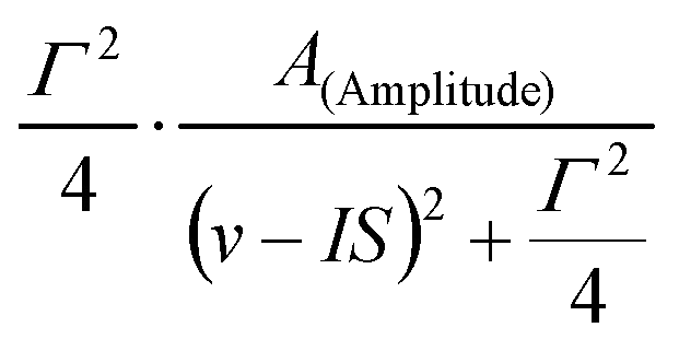
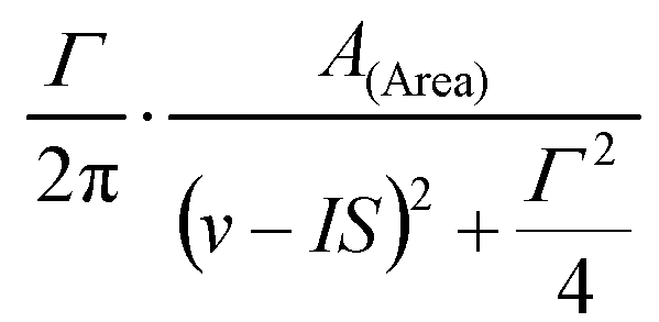
• Lorentzian (LOR) - Lorentzian peak shape described by three parameters, A (denoting either the amplitude or the area of the peak), IS (denoting the center of the peak), and Γ (denoting the FWHM of the peak). Depending om whether Amplitude or Area mode is selected, the peak is calculated as

Amplitude mode	Area Mode

 
• Pseudo-Voigt (PVOI) - Approximation of the Voigt line profile, calculated as described in J. APPL. CRYST. 19 (1986) 63. When the Pseudo-Voigt line shape is selected for a subspectrum, then the former line width parameter(s) will determine the line width (FWHM) of the associated Gaussian profile(s), whereas the Lorentzian line width (being common to all the peaks belonging to the same subspectrum) is added as an additional parameter to the parameter list of the subspectrum in question.
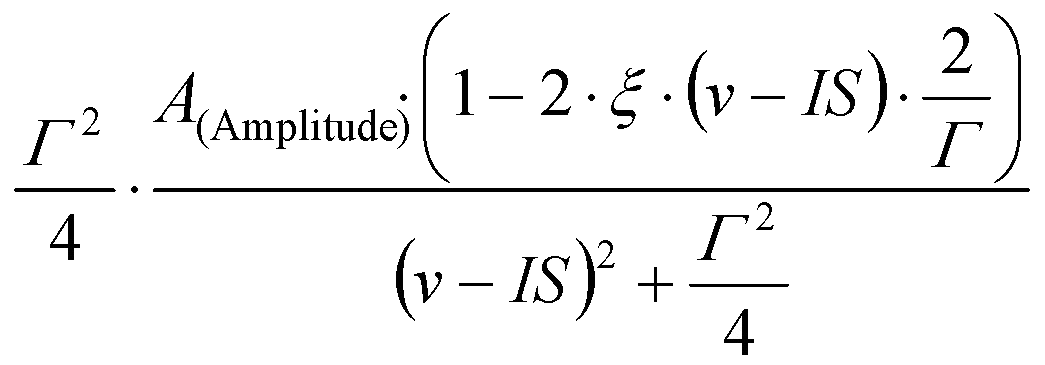
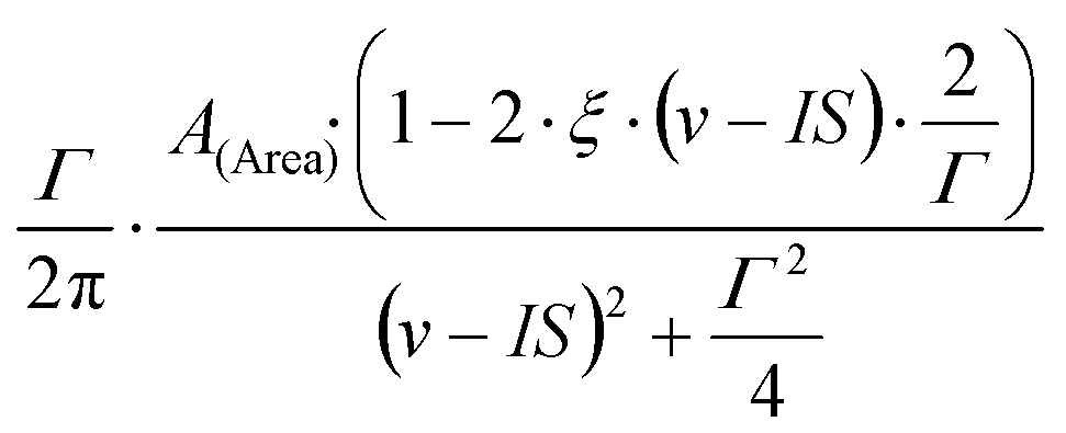
• Lorentzian with dispersion (LOR-DI) - Peak shape that takes into account the interference effect between nuclear and atomic absorption of γ-rays (see PRL 28 (1972) 530 and PRC 8 (1973) 1916 for details), described by four parameters, A (denoting either the amplitude or the area of the peak), IS (denoting the center of the peak), Γ (denoting the FWHM of the peak) and ξ (denoting the dispersion amplitude):

  Amplitude mode	Area Mode

   
  When Lorentzian with dispersion is selected as peak shape for one of the subspectra, then the ξ dispersion amplitude (being common to all the subspectra belonging to the same spectrum) is added as an additional parameter to the parameter list of the background.


• Lorentzian with cosine smearing (LOR-CS) - Peak shape that takes into account the cosine-broadening effect caused by non-ideal geometrical conditions. The peak shape is calculated as described in Hyp. Int. 29 (1986) 1539. When this line shape is selected for a subspectrum, a new parameter named Visual angle [deg], denoting the visual angle of the absorber or the detector aperture (which is smaller depending on the actual geometrical conditions) viewed from the center of the source, is added to the parameter list of the subspectrum in question. In the case of a Lorentzian with cosine smearing, the amplitude, area and percentage values displayed or printed by MossWinn are exactly those which one would get for the corresponding Lorentzian without cosine smearing. That is (apart from possible f-factor differences) subspectrum relative areas in this case also reflect the relative occurrence of Mossbauer nuclides in different microenvironments. At the same time the area values are not equal to the corresponding apparent (measured and fitted) spectral area.

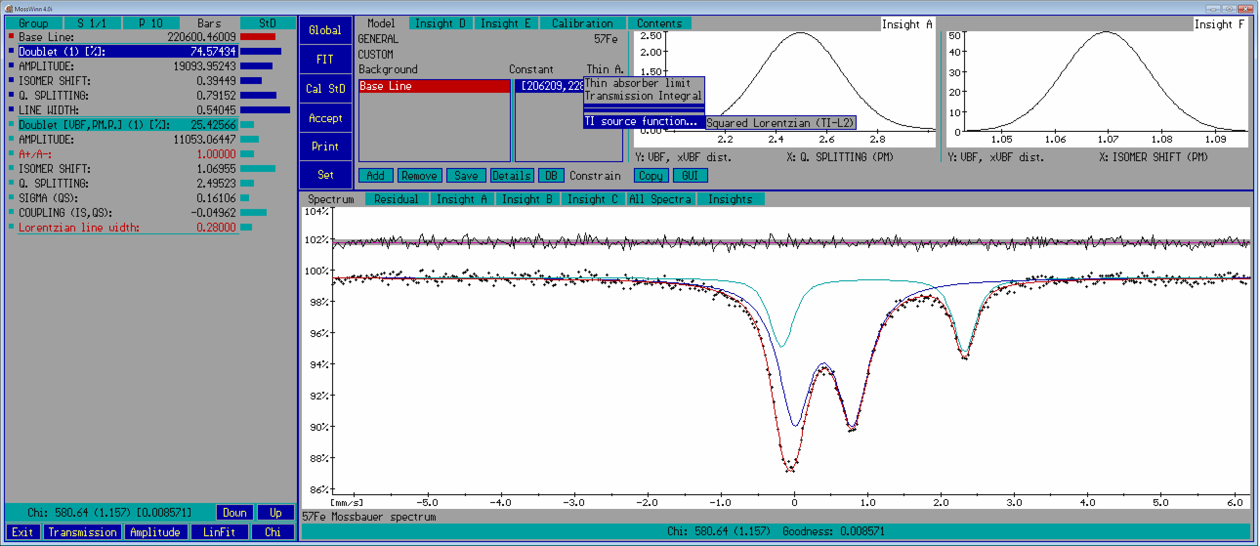
• Thin absorber limit (Thin A.) / Transmission Integral (T-INT) / TI source function... (TI-L2) - Press on this popup box in order to choose between thin absorber approximation and transmission integral modes. When transmission integral mode is selected, the necessary additional parameters (Background fraction, Effective Thickness, Source f factor, Source Line Width) are automatically added to the parameter list of the background. In transmission integral mode, the usual subspectrum line widths denote absorber line widths. 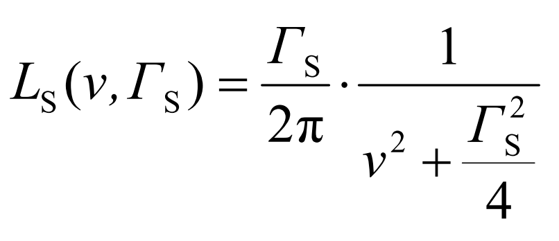In the different transmission integral modes, the source line shape is expressed as follows (Γ_s denotes the source line width):

Transmission Integral Mode	Source line shape
T-INT
TI-L2 (Concerning this option see Phys. Rev. A 84 (2011) 053851.)

• Background options - Press on this popup box in order to select one of the available background function options:

• Constant
• Slope
• Curvature
• Third Order
• Unfolded
• Unfolded + Slope

• Add - The Add menu box provides access to functions related to the following kinds of addition operations.

• New Subspectrum - This menu provides access to subspectrum models saved earlier via the Save Subspectrum menu option. Select one of the subspectrum models in order to add a corresponding subspectrum to the current fit model. Subspectra are listed by their entry names that may be different from the actual name given to the subspectrum when it is added to the current model. If a subspectrum with the same name already exists, then the name of the new subspectrum will be made unique by numbering. Press on the New Subspectrum menu item in order to add a singlet to the current model. Note that subspectra that are already part of the fit model can be duplicated by turning to the Add one more subspectrum of this type option of their headline menu.
• New Subspectrum (DLL) - This menu provides access to subspectrum models available in — user programmed and compiled — dynamic link libraries being saved in the code library directory with a name corresponding to the mask SUB*.DLL. (DLL libraries are listed here only if they were enabled in the SET menu.) Select one of the subspectrum models in order to add a corresponding subspectrum to the current fit model.
• New Subspectrum Group - This menu provides access to subspectrum group models saved earlier via the Save Subspectrum Group... menu option. Select one of the subspectrum group models in order to add a corresponding subspectrum group to the current fit model. Subspectrum groups are a collection of several subspectra that may be connected to eachother by user-defined constraints. A subspectrum group can also be used to model a phase whose Mossbauer spectrum consists of more than one subspectrum. For example, at room temperature the phase magnetite may be modeled by two sextets having an area ratio of 2:1 corresponding to iron atoms at octahedral and tetrahedral sites, respectively. Thus, room-temperature magnetite may be described by a subspectrum group consisting of two sextets with a fixed area ratio of 2:1.
• New Shared Subspectrum - Turn to this option in order to add the selected subspectrum (as a shared subspectrum) to all the fit models fitted simultaneously.
• New Shared Subspectrum (DLL) - Turn to this option in order to add the selected DLL subspectrum (as a shared subspectrum) to all the fit models fitted simultaneously.
• New Shared Subspectrum Group - Turn to this option in order to add the selected subspectrum group (as a group of shared subspectra) to all the fit models fitted simultaneously.
• Extra Fit Parameter - Turn to this option in order to add an extra (custom) fit parameter to the parameter list of the background. Extra parameters may be used to describe experimental variables of the measurement, e.g. temperature, external magnetic field, sample orientation etc. Fit models may be made to depend on the extra parameters such that theoretical dependencies may be taken into account. For example, isomer shift parameters may be enforced to decrease linearly with temperature thereby modeling (approximately) the effect of the second order doppler shift at higher temperatures. (Dependency functions of arbitrary complexity can be defined by modifying the DEP_DLL1.PAS source and compiling it to observe a new DEP_DLL1.DLL dynamic link library.) The value of fit parameters can also be examined/tabulated as a function of extra parameters: for example, the value of a hyperfine magnetic field parameter may be depicted as a function of temperature or external magnetic field on one of the insight pages.
• New Spectrum to fit - Turn to this option in order to add one or more new spectra (selected among those being loaded on the current desk in the main menu) to the fit. Spectra added to the fit are all fitted simultaneously. For the newly added spectra the fit model set for the current spectrum will be initiated. To remove a spectrum from the list of simultaneously fitted spectra, turn to the Remove menu box.

• Remove - The Remove menu box provides access to functions related to the following kinds of removal operations.

• Subspectrum - Turn to this option in order to remove one of the shared or unshared subspectra from the fit model. A shared subspectrum can be removed from the current model as well as from models set for other simultaneously fitted spectra.
• All subspectra / for all the fitted spectra - Turn to this option in order to remove all shared and unshared subspectra from the fit model associated with the current spectrum. Select the appearing submenu item in order to carry out the same operation for all the simultaneously fitted spectra.
• Spectrum from fit - Turn to this option in order to remove one of the spectra from a simultaneous fit.
• Subspectrum from collection - Turn to this option in order to delete one of the subspectra saved earlier via the Save Subspectrum menu option to the subspectrum collection.
• Subspectrum Group from collection - Turn to this option in order to delete one of the subspectrum groups saved earlier via the Save Subspectrum Group... menu option.
• Fit model from model group - Turn to this option in order to delete one of the fit models (of the current model group) saved earlier via the Save Model As menu option.
• Model group - Turn to this option in order to delete one of the model groups with all of its models.
• FitLog file - Turn to this option in order to delete the HTML FitLog file created earlier for the current spectrum.
• Parameter - Turn to this option in order to delete one of the parameters of the currently selected subspectrum.

• Save - The Save menu box provides access to functions related to the following kinds of save operations.

• Save Subspectrum - Turn to this option in order to save one of the subspectra to the subspectrum collection. The name of the subspectrum (as displayed by the subspectrum headline) as well as its entry name (by which it is identified in the subspectrum collection) can be defined after the subspectrum is selected. Turn to the Add menu box in order to add the saved subspectrum to a fit model.
• Save Subspectrum Group... - Turn to this option in order to save two or more subspectra of the current model as a subspectrum group. The individual subspectra will be saved with their current name. The constraints (if any) among the parameters of the saved subspectra will be preserved in the saved subspectrum group. Turn to the Add menu box in order to add the saved subspectrum group to a fit model.
• Save Model As - Turn to this option in order to save the current model to an existing or to a newly created model group. The saved model can be reloaded either via the Models popup box or the Model groups popup box.
• Save HTML FitLog - Turn to this option in order to save an additional HTML FitLog to the FitLog file of the current spectrum, according to the current state of the fit. The FitLog file is located/created in the folder that contains also the corresponding spectrum data file. Its name is derived from the file name of the latter via the addition of .log.htm . Multiple FitLogs can be saved to a single FitLog file. MossWinn takes care of duplicates: it will not add a new FitLog if it is essentially identical with one being already present in the FitLog file. The FitLog file can be opened by pressing on the gray info line popup box directly below the spectrum graph area. To access the functions related to the FitLog file, press with the right mouse button on the Accept menu box.
• Save Spectrum - Turn to this option in order to save an independent copy of the current spectrum with an arbitrary path and name. (The fit will continue with the original spectrum.)
• Save Insight Page... - Turn to this option in order to save the content of one of the active insight pages as a textual data file.

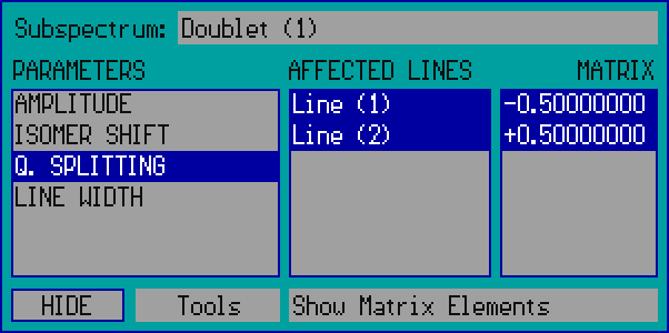
• Details - Press on the Details menu box in order to invoke the Details panel that provides access - among others - to the matrix elements influencing the amplitudes, positions and widths of the peaks contributing to a linear model. For details press on one of the visual elements on the image below.

• Subspectrum - Press on this popup box to select the subspectrum to handle.
• Parameters - This box lists the parameters associated with the selected subspectrum. Press on any of the parameter names in order to select it, and to have the lines affected by the parameter in question become selected in the list on the right.
• Affected lines - This box lists the Lines (peaks) associated with the selected subspectrum. The Lines affected by the selected parameter are displayed blue-selected. In case of Amplitude and Line Width type parameters press on any of the Lines to have it selected/deselected. The number and name of the corresponding Amplitude and Line Width type parameters will be adjusted automatically as needed.
• Matrix - This box lists the matrix elements associated with the selected parameter. The matrix elements reflect how the selected amplitude/position/width type parameter affects the amplitude/position/width of the absorption peaks associated with the subspectrum. For example the case shown above reflects that the value of the quadrupole splitting parameter is multiplied by -0.5 / +0.5 before the result is added to the position of Line (1) / Line (2). Press on any of the matrix elements in order to edit the corresponding value.
• Hide - Press on the Hide box in order to hide the details panel.
• Tools - Press on the Tools popup box in order to alter the linear model - associated with the selected subspectrum - via the following options.
• Add Position Type Parameter - Turn to this option in order to add a position type parameter to the linear model.
• Remove Position Type Parameter - Turn to this option in order to remove one of the position type parameters of the linear model.
• Add Absorption Line - Turn to this option in order to add an absorption line to the linear model.
• Remove Absorption Line - Turn to this option in order to remove one of the absorption lines of the linear model.
• Functions popup box - Press on this popup box in order to access the following functions of the details panel.
• Show Matrix Elements - Select this option in order to have the details panel display the affected lines and the matrix elements associated with the selected parameter, as in the example shown above.
• Show Enabled Intervals - Select this option in order to have the details panel display the enabled intervals associated with the selected parameter. The enabled intervals are calculated on the basis of the constraints displayed in the Parameter constraints list box.
• Show Internal Values - Select this option in order to have the details panel display the current value of internal program variables associated with the selected subspectrum and parameter. The details of this feature are not documented: during development/testing it is used by the author to monitor the internal state of some relevant program variables.

• DB - The DB menu box provides access to functions related to the MossWinn Internet Database (MIDB).

• Find and apply best match - Turn to this option in order to search through the database records in order to find the spectrum that best matches the fitted spectrum currently on the screen, and to set the corresponding fit model as included in the database record returned by the search. (The currently set fit model will be overwritten.) The fitness of the database records with respect to the current spectrum is evaluated by considering the isomer shift of the isomer shift reference material (associated with the current source nuclide) that can be set via the Isomer shift reference submenu option of the SET menu. The search can be performed via the following submenu options (a press directly on the Find and apply best match menu item is equivalent to the option Considering own records):
• Considering own records - The search will consider only those records that were published in the database by using the hardware key that is currently attached to the computer.
• Considering all records - The search will consider all database records.
• Considering all transmission (reflection) type records - The search will consider only those database records that refer to measurements carried out in transmission (reflection) geometry.
• The fit model returned as the best match will be saved automatically as a new model of the MIDB [ * ] model group where * stands for the corresponding source nuclide. Apart from the best match, the search will also return several further records in descending order of the fitness of their included fit model with respect to the spectrum under analysis. Select this menu again in order to see the corresponding list and apply another one of the returned records.
• Open compound class in database browser - Turn to this option in order to select one of the records returned by the Find and apply best match function, and open the corresponding compound class in the database browser.
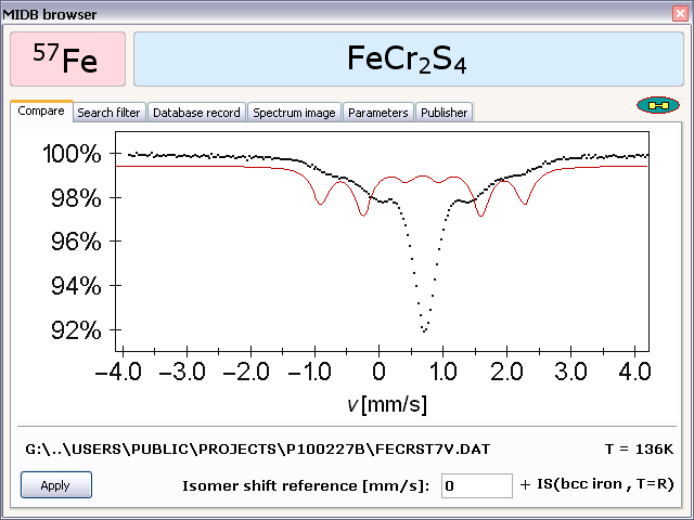
• Browse the internet database - Select this option in order to display the database browser that allows one to search through the database records according to various criteria. The database browser also provides the possibility to try/apply the fit models, represented by the database records, to the fitted spectrum currently on the screen.
• Publish record in the internet database - Select this option in order to publish the current fit model and/or a downsampled version of the current spectrum in the MossWinn Internet Database. If along with the fit parameters you also want to publish their standard deviation in the database, calculate the corresponding standard deviations via the Cal StD menu before turning to this option. Once the option is selected, first the Database record input form becomes displayed on which one can set various parameters associated with the record to be published. Then, the next form provides the possibility to set the resampled form of the measured spectrum, and to declare whether one wants to publish only the fit model, only the resampled spectrum, or both. On the next form a preview of the record is displayed, where one can check how the record will appear when published. The record becomes finally published when on the preview form the Publish record button is pressed. Once a record is published in the database, it may appear in the MIDB database browser of MIDB subscribers all around the world. The MIDB Publisher's Guide contains useful information on recommended practices concerning the publication of MIDB records.
• Withdraw record from the internet database - Select this option in order to withdraw a MIDB record published earlier by using the hardware key that is currently attached to the computer ( own record ). The own record that is to be withdrawn can be selected on the appearing form. Withdrawal of own records from the MIDB database does not require subscription to the database.
• Edit record published in the internet database - Select this option to edit one of the own MIDB records by changing the record parameters that can be set on the Database record input form. The fit model and the resampled spectrum associated with the record cannot be edited in this way. The own record that is to be edited can be selected on the appearing form.
• Synchronize local data with the internet database - Select this option to carry out pending MIDB publication and withdrawal operations, and to synchronize local data with the MIDB host server. The frequency of such synchronization events may be subject to a limitation.
• Open MIDB Compound Summary in the default browser - Select this option to open the MIDB Compound Summary in the default browser.
• Help on the DB menu box - Select this option to bring up this html help concerning the DB menu box.

• Constrain - Press on the Constrain popup box in order to declare a new constraint for the selected fit parameter. Some of the constraints take effect immediately, others are effective only during fitting. The local fit procedure obeys these latter constraints only if they are designated to be HARD constraints. Also, HARD constraints take effect immediately. Some of the constraints are initialized without being made active. Inactive constraints are listed without blue highlight in the Parameter constraints list box. Press on them with the right mouse button in order to make them active.

• Distribution (available only for position type parameters) - Declare a position type parameter to be of the distribution type in order to fit a distribution in the selected parameter (distribution parameter). For example hyperfine magnetic field distribution, quadrupole splitting distribution or isomer shift distribution can be fitted in this way. In order to declare correlations, constrain another parameter(s) to depend linearly on the distribution parameter. The distribution curve can be made to be displayed (example) on either of the insight pages. The following distribution types are available:
• Unrestricted (UNR) - The distribution is calculated as described in J. Phys. E: Sci. Instrum. 7 (1974) 526. The distribution curve can take on negative values as well.
• Positive, Free Boundaries (PFB) - Similar to the previous case, but the distribution cannot take on negative values.
• Positive, Zero Left Boundary (PZLB) - The distribution cannot take on negative values, and it goes to zero at its left boundary.
• Positive, Zero Right Boundary (PZRB) - The distribution cannot take on negative values, and it goes to zero at its right boundary.
• Positive, Zero Left & Right Boundaries (PZLRB) - The distribution cannot take on negative values, and it goes to zero at its both boundaries.
• Split distribution - Select this option in order to split the distribution at some intermediate value by adding the SPLIT [x] directive to the parameter constraints list box, where x denotes an intermediate distribution-parameter value. As a result, the distribution will contribute to the fitting curve by two separate subspectra: one belonging to distribution-parameter values higher than x, and the other belonging to distribution-parameter values lower than or equal to x.
• When distributions are fitted in conjunction with transmission integral fitting then the parameter Filter cutoff is automatically added to the parameter list of the background. This parameter controls the level of noise filtering necessary for the calculations. Its value is constrained to the interval of [0,1]. A Filter cutoff value of 1.0 means hardly any filtering, whereas a value of 0.0 means strongly suppressed noise level. The Filter cutoff parameter should be fitted in order to achieve optimal results. See the manual and corresponding publications for further details.
 
• Relative (available only for amplitude type parameters) - Constrain an amplitude type parameter to be relative in order to fit its relative value compared to another parameter. If the amplitude type parameter - that is constrained to be relative - is the first amplitude type parameter in its subspectrum, then its absolute value is calculated as the product of its relative value and the Base Line parameter of the background. Otherwise, the absolute value is calculated as the product of the relative value and the absolute value of the subspectrum's first amplitude type parameter. For example, declaring the amplitude of the 2nd and 5th lines of a ⁵⁷Fe sextet to be relative enables one to set the amplitude of the 2nd and 5th lines relative to that of the 3rd and 4th. In order to remove the Relative constraint, remove the word RELATIVE from the corresponding list of constraints.
 
• Is Equal to - The parameter should remain equal to the value that is to be given in the Parameter constraints list box.
• Is in the Range - The parameter should remain inside the range that is to be given in the Parameter constraints list box.
• INClude Range - The parameter should be allowed to take on values from the range that is to be given in the Parameter constraints list box. This constraint can be used to modify the effect of other constraints.
• EXClude Range - The parameter should not be allowed to take on values from the range that is to be given in the Parameter constraints list box. This constraint can be used to modify the effect of other constraints.
• Higher Than - The parameter should exceed the value that is to be given in the Parameter constraints list box. This constraint can be used to modify the effect of other constraints.
• Higher or Equal - The parameter should not be less than the value that is to be given in the Parameter constraints list box. This constraint can be used to modify the effect of other constraints.
• Less Than - The parameter should be less than the value that is to be given in the Parameter constraints list box. This constraint can be used to modify the effect of other constraints.
• Less or Equal - The parameter should not exceed the value that is to be given in the Parameter constraints list box. This constraint can be used to modify the effect of other constraints.
• Hard constraint - The above type of constraints declared for the selected parameter should be obeyed also by the local fit procedure. Otherwise these constraints are taken into account only by the Global fitting procedure.
 
• Higher Than #PARAMETER - The parameter should exceed the one selected in the appearing submenu list.
• Higher or Equal #PARAMETER - The parameter should not be less than the one selected in the appearing submenu list.
• Less Than #PARAMETER - The parameter should remain below the one selected in the appearing submenu list.
• Less or Equal #PARAMETER - The parameter should not exceed the one selected in the appearing submenu list.
• Not Equal to #PARAMETER - The parameter should not be equal to the one selected in the appearing submenu list.
• Is Close to #PARAMETER - The parameter should remain close to the one selected in the appearing submenu list. What is close and what is far is determined by the allowed parameter range of the latter parameter.
• Is Far from #PARAMETER - The parameter should remain far from the one selected in the appearing submenu list. What is close and what is far is determined by the allowed parameter range of the latter parameter.
 
• := #PARAMETER - The parameter should be equal to the one selected in the appearing submenu list. In order to remove the constraint, in the parameters' panel press on the name of the constrained parameter (displayed by brown color).
• := #PARAMETER + CONST - The parameter should be equal to the one selected in the appearing submenu list plus another, newly created parameter, which latter will be added to the parameter list of the subspectrum of the constrained parameter with the name b {NAME} where NAME is the name of the constrained parameter. In order to remove the constraint, in the parameters' panel press on the name of the constrained parameter (displayed by brown color).
• := #PARAMETER * CONST - The parameter should be equal to the product of the one selected in the appearing submenu list and another, newly created parameter, which latter will be added to the parameter list of the subspectrum of the constrained parameter with the name m {NAME} where NAME is the name of the constrained parameter. In order to remove the constraint, in the parameters' panel press on the name of the constrained parameter (displayed by brown color).
• := #PARAMETER * CONST1 + CONST2 - The parameter should depend linearly on the one selected in the appearing submenu list. The linear coefficient and the constant term will be added to the parameter list of the subspectrum of the constrained parameter as newly created parameters with the name m {NAME} and b {NAME}, respectively, where NAME is the name of the constrained parameter. In order to remove the constraint, in the parameters' panel press on the name of the constrained parameter (displayed by brown color).
 
• := SMOOTH MONOTONIC ( #PARAMETER ) - The parameter should depend via the following — smooth and monotonic — function on the parameter (x) selected in the appearing submenu list:
  

  Smooth monotonic function	Examples

  The x_center, y_from, y_to and Steepness parameters will be added to the parameter list of the subspectrum of the constrained parameter as newly created parameters with the names Center X {NAME}, From Y {NAME}, To Y {NAME} and Steepness {NAME}, respectively, where NAME is the name of the constrained parameter. In order to remove the constraint, in the parameters' panel press on the name of the constrained parameter (displayed by brown color). This option can be used to set up a versatile constraint that can ensure the smooth, monotonic (increasing or decreasing) dependence of the currently selected fit parameter (y) on a physical parameter (x) such as the temperature of the sample, but may also model a step-like transition of a parameter as the function of another one. The option requires either the DBM version of MossWinn or subscription to the MossWinn services.
 
• := SMOOTH WITH SLOPE ( #PARAMETER ) - The parameter should depend via the following — smooth, but not necessarily monotonic — function on the parameter (x) selected in the appearing submenu list:
  

  Smooth function with slope	Examples

  The x_center, y_from, y_to, Steepness and Slope parameters will be added to the parameter list of the subspectrum of the constrained parameter as newly created parameters with the names Center X {NAME}, From Y {NAME}, To Y {NAME}, Steepness {NAME} and Slope {NAME}, respectively, where NAME is the name of the constrained parameter. In order to remove the constraint, in the parameters' panel press on the name of the constrained parameter (displayed by brown color). This option can be used to set up a versatile constraint that can ensure the smooth dependence of the currently selected fit parameter (y) on a physical parameter (x) such as the temperature of the sample, but may also model a step-like transition of a parameter as the function of another one. The option requires either the DBM version of MossWinn or subscription to the MossWinn services.
 
• := User Programmed Function [ Cubic ] - The parameter should depend on the one selected in the appearing submenu list as determined by the - arbitrary - function included in the DEP_DLL1.DLL dynamic link library. (By default this is a cubic function.) The necessary number of additional parameters will be added to the parameter list of the subspectrum of the constrained parameter as newly created parameters with names determined by the functions in the DLL. In order to remove the constraint, in the parameters' panel press on the name of the constrained parameter (displayed by brown color).
 
• := #Percentage constrained - Select this option in order to constrain the spectral area of the selected subspectrum by a percentage parameter that determines the relative spectral area of the subspectrum. The newly created percentage parameter will be added to the parameter list of the subspectrum whose area is constrained. In order to remove the percentage constraint, in the parameters' panel press on the name of the first amplitude type parameter (displayed by brown color) of the constrained subspectrum.

• Copy - The Copy menu box provides access to various copy-to-clipboard functions as detailed below.

• All spectra (as image) - to copy all simultaneously fitted spectra to the clipboard as a single image (example). The spectra will follow each other according to the spectrum order set previously via the spectrum number popup box. The resolution of the image can be set via the Printer Setup Dialog with Clipboard - multiple spectra selected as printer.
• All spectra (as text) - to copy all simultaneously fitted spectra to the clipboard as text, with the velocity values, the measured data, the fit envelope and the subspectra included as comma delimited columns. The spectra will follow each other according to the spectrum order set previously via the number of spectra popup box. This option may be used to export numerical data from MossWinn for use in external data processing & graphics software.
• All spectra (as xls) - to make a copy of all the simultaneously fitted spectra, all the valid insight pages, the fit results in two different tabular forms as well as the fit reports associated with the current state of the fit in the form of a single XLS spreadsheet file, in which the different spectra/insight pages/tables and the fit reports appear on separate worksheet pages (example). This option provides a convenient way to collect the numerical data of the current state of the fit in a single XLS file for backup, graph creation or publication purposes. In order to have the standard deviation of fit parameters included in the XLS file, turn to the Cal StD function before selecting this option. Once created, MossWinn attempts to open the XLS file with an associated software application. Access to this option requires subscription to the MossWinn Services. For further details click here.


• Current spectrum (as image) - to copy the currently displayed spectrum to the clipboard as image. The resolution of the image can be set via the Printer Setup Dialog with Clipboard - single spectrum selected as printer.
• Current spectrum (as text) - to copy the currently displayed spectrum to the clipboard as text, with the velocity values, the measured data, the fit envelope and the subspectra included as comma delimited columns. This option may be used to export numerical data from MossWinn for use in external data processing & graphics software.
• Current spectrum (as xls) - to copy the currently selected fitted spectrum, the corresponding fit results in two different tabular forms as well as the associated fit report in the form of a single XLS spreadsheet file, in which the spectrum data, the fit result tables and the fit report appear on separate worksheet pages (example). In order to have the standard deviation of fit parameters included in the XLS file, turn to the Cal StD function before selecting this option. Once created, MossWinn attempts to open the XLS file with an associated software application. Access to this option requires subscription to the MossWinn Services. For further details click here.


• All insight pages (as image) - to copy all the valid insight pages to the clipboard as a single image.
• All insight pages (as text) - to copy the numerical data (including parameter standard errors if calculated) of all the valid insight pages to the clipboard as text. This option may be used to export numerical data from MossWinn for use in external data processing & graphics software.
• All insight pages (as xls) - to make a copy of the numerical data of all the valid insight pages in the form of a single XLS spreadsheet file, in which the data of the different insight pages appear on separate worksheets (example). In order to have standard deviation of fit parameters included in the XLS file, turn to the Cal StD function before selecting this option. Once created, MossWinn attempts to open the XLS file with an associated software application. Access to this option requires subscription to the MossWinn Services. For further details click here.


• Insight page (as image)... - to copy a selected insight page to the clipboard as a single image.
• Insight page (as text)... - to copy the numerical data of a selected insight page to the clipboard as text. This option may be used to export numerical data from MossWinn for use in external data processing & graphics software.
• Insight page (as xls)... - to make a copy of the numerical data of the selected insight page in the form of an XLS spreadsheet file (example). In order to have standard deviation of fit parameters included in the XLS file, turn to the Cal StD function before selecting this option. Once created, MossWinn attempts to open the XLS file with an associated software application. Access to this option requires subscription to the MossWinn Services. For further details click here.


• Fit report for the current spectrum - to copy the results concerning the currently displayed spectrum to the clipboard in the fit report text format (example).
• Fit report for all the fitted spectra - to copy the fit results of all the simultaneously fitted spectra to the clipboard in the fit report text format. The spectra will follow each other according to the spectrum order set previously via the spectrum number popup box.


• Fit results as table (with spectra in rows)... - to copy the numerical results concerning all of the simultaneously fitted spectra into the clipboard as comma delimited numerical data in rows, each of which corresponds to a single spectrum. This option may be used to export numerical data from MossWinn for use in external data processing & graphics software. Concerning the format of the standard deviation values, one of the following options can be chosen:
• with StD values in separate columns
• with StD values in parentheses after values
• with StD values in parentheses as error in last digit(s)
• Fit results as table (with spectra in columns)... - to copy the numerical results concerning all of the simultaneously fitted spectra into the clipboard as comma delimited numerical data in columns, each of which corresponds to a single spectrum. This option may be used to export numerical data from MossWinn for use in external data processing & graphics software. Concerning the format of the standard deviation values, one of the following options can be chosen:
• with StD values in separate rows
• with StD values in parentheses after values
• with StD values in parentheses as error in last digit(s)


• Correlation matrix... - to copy the correlation matrix of the fit to the clipboard. The following options are available:
• As image (for all spectra)
• As image (for current spectrum)
• As image (value limited, for all spectra)
• As text (for all spectra)
• As text (for current spectrum)
• As text (value limited, for all spectra)

• GUI - The GUI (graphical user interface) menu box provides the possibility to change MossWinn's internal screen resolution according to the following options.

• 800 x 400 - to set the internal MossWinn screen resolution to 800 x 400.
• 800 x 450 - to set the internal MossWinn screen resolution to 800 x 450.
• 800 x 500 - to set the internal MossWinn screen resolution to 800 x 500.
• 800 x 650 - to set the internal MossWinn screen resolution to 800 x 650.
• 900 x 450 - to set the internal MossWinn screen resolution to 900 x 450.
• 900 x 500 - to set the internal MossWinn screen resolution to 900 x 500.
• 900 x 650 - to set the internal MossWinn screen resolution to 900 x 650.


• Set optimum resolution for full screen mode - to set the internal MossWinn screen resolution equal to a value that is optimum for full screen mode by considering the full resolution of the current screen.
• Set optimum resolution when entering full screen mode - when selected, the internal MossWinn screen resolution is automatically set to be equal to a value that is optimum for full screen mode whenever the latter is entered by pressing F4. When full screen mode is entered with this option being unselected, the program sets the internal resolution to the one last used in full screen mode.


• 960 x 540 (Optimum for FHD full screen) - to set the internal MossWinn screen resolution to 960 x 540, which is considered to be optimum in full screen mode on a FHD (1920 x 1080) screen.
• 960 x 600 (Optimum for WUXGA full screen) - to set the internal MossWinn screen resolution to 960 x 600, which is considered to be optimum in full screen mode on a WUXGA (1920 x 1200) screen.
• 1280 x 540 (Optimum for UW-UXGA full screen) - to set the internal MossWinn screen resolution to 1280 x 540, which is considered to be optimum in full screen mode on an UW-UXGA (2560 x 1080) screen.
• 1280 x 720 (Optimum for QHD & 4K HD full screen) - to set the internal MossWinn screen resolution to 1280 x 720, which is considered to be optimum in full screen mode on QHD (2560 x 1440) and 4K HD (3840 x 2160) screens.
• 1720 x 720 (Optimum for UW-QHD full screen) - to set the internal MossWinn screen resolution to 1720 x 720, which is considered to be optimum in full screen mode on an UW-QHD (3440 x 1440) screen.
• 1920 x 1080 (Alternative for FHD and 4K HD full screen) - to set the internal MossWinn screen resolution to 1920 x 1080, which is considered as a higher resolution alternative on FHD (1920 x 1080) and 4K HD (3840 x 2160) screens.


• Set maximum resolution for full screen mode - to set the internal MossWinn screen resolution to its maximum value considering the full resolution of the current screen. This option is available only when the program is in full screen mode.

• Coupled W. - Put a check on this box in order to make all the lines of a linear model to have the same line width. Clear the check box in order to set up independent line width parameters (2 in the case of doublets, 3 in the case of sextets) determining the line widths of the lines. This option is available only for doublet and sextet linear models of the nuclides ⁵⁷Fe, ¹¹⁹Sn and ¹²⁵Te. The check box can be invoked via the Subspectrum matrix elements option of the Contents tab that is accessible in high screen resolution mode.

• Texture - Put a check on this box in order to lift powder constraints of a linear (doublet or sextet) powder geometry model by inserting one additional amplitude type parameter into the model of the selected subspectrum. Clear the check box to return to the constraints of powder geometry. This option is available only for doublet and sextet linear powder geometry models of the nuclides ⁵⁷Fe, ¹¹⁹Sn and ¹²⁵Te. The check box can be invoked via the Subspectrum matrix elements option of the Contents tab that is accessible in high screen resolution mode.

• Enable neg. amplitudes - Put a check on this box in order to enable amplitude parameters to take on negative values. Normally, amplitude type parameters are forced to be non-negative.

• Contents - click on the Contents tab in order to set the contents of the extra screen area that becomes available on the Model page in high screen resolution modes. Depending on the size of the screen area in question, one or more of the following elements can be made to be displayed.

• Parameter enabled intervals (with the check box Enable neg. amplitudes)
• Subspectrum matrix elements (with the check boxes Coupled W. and Texture)
• Insight A
• Insight B
• Insight C
• Insight D
• Insight E
• Insight F

The selected elements are displayed from left to right in the above order. When the available horizontal space is not sufficient to display more elements, the remaining selected elements become skipped. The possible functions of the insight pages are listed here.

• Calibration - click on the Calibration tab in order to access the calibration page that allows the calibration of the velocity axis of spectra with known position type parameters (mainly the isomer shift, the hyperfine magnetic field and/or the quadrupole splitting).

• Source - Source nuclide that was used to measure the calibration spectrum. In the present version only ⁵⁷Fe Mossbauer spectra can be used to calibrate the velocity axis.
• Matrix - Source matrix that was used to measure the calibration spectrum. Built in matrices include

• Rhodium - with ⁵⁷Fe isomer shift of +0.114 mm/s relative to α-iron.
• Chromium - with ⁵⁷Fe isomer shift of –0.154 mm/s relative to α-iron.
• Palladium - with ⁵⁷Fe isomer shift of +0.177 mm/s relative to α-iron.

Turn to the menu option Define Matrix... in order to define further - single line - matrices by declaring their name and isomer shift relative to α-iron.

• Absorber - Absorber material with known position type parameters, whose ⁵⁷Fe Mossbauer spectrum was measured in order to calibrate the velocity axis. Absorption materials built in for calibration purposes include

• Alpha Iron - α-Fe with ⁵⁷Fe isomer shift of 0.0 mm/s and hyperfine magnetic field of 33 T.
• Alpha Iron + SS - α-Fe measured together with stainless steel.
• Alpha Iron + SNP - α-Fe measured together with sodium nitroprusside (SNP).
• Alpha Iron + SNP + SS - α-Fe measured together with SNP and SS (resulting in 1 sextet + 1 doublet + 1 singlet).
• SNP + SS - SNP measured together with SS.
• Sodium Nitroprusside (SNP) - sodium nitroprusside (SNP) with ⁵⁷Fe isomer shift of –0.26 mm/s relative to α-Fe and quadrupole splitting of +1.7034 mm/s.
• Stainless steel (SS) - stainless steel (SS) whose ⁵⁷Fe isomer shift is –0.09 mm/s relative to α-Fe.

Note that during calibration fitting the fixed isomer shift values are always meant relative to the source matrix. In order to define further absorber fit models for the sake of velocity scale calibration, set the appropriate fit model (on the Model tab) with fixed position type parameters including isomer shift values relative to α-iron, and then by pressing on the Absorber popup on the Calibration tab turn to the menu option Define Absorber....

• Isomer shift reference - Press on this popup box in order to set the reference material for the isomer shift. This setting is taken into account when the calibration fit is accepted. Spectra - calibrated on the basis of the fitted calibration spectrum - when fitted will display isomer shift values relative to the reference material selected here. If the calibration spectrum is used to calibrate the velocity axis of ⁵⁷Fe Mossbauer spectra, then Alpha Iron is the recommended reference material. When the ⁵⁷Fe calibration spectrum is used to calibrate the velocity axis of spectra measured with a source nuclide other than ⁵⁷Fe, then Source material is the recommended reference. In the latter case the velocity axis will be calibrated with absolute velocity values, i.e. the velocity value attributed to a particular channel will be equal to the actual velocity the source was moving with relative to the absorber when the counts in the channel in question were collected. Spectra calibrated in this way will display isomer shift values relative to that of the source material (e.g. ¹⁵¹SmF₃ if such a source was used to measure a ¹⁵¹Eu Mossbauer spectrum).
• Velocity waveform - Put a check on the velocity waveform that was used to measure the calibration spectrum. Triangle and Sinusoid refer to the two most often applied waveforms. In the case of folded calibration spectra the Triangle waveform is equivalent to the usual linear velocity scale.
• Folded / Unfolded - Put a check on Folded if the calibration spectrum is a folded spectrum. MossWinn is able to calibrate and fit unfolded spectra as well. In such a case the unfolded calibration spectrum has to be used to calibrate the velocity axis. Put a check on Unfolded in order to calibrate the velocity axis of an unfolded calibration spectrum (e.g. 2×6 peaks of α-iron).
• Sign of first-channel velocity - Put a check on Negative if the first data count in the data file associated with the calibration spectrum can be attributed to negative source velocity. Otherwise, put a check on Positive. An invalid setting here will result either in an unsatisfactory fit, or in an unrealistic high (considerably higher than 1.0) absolute value of the Delay [Dwell Time] parameter.
• Calibration mode Active / Inactive - Put a check on Active in order to let the calibration settings determine the velocity axis and start calibration fitting. Put a check on Inactive in order to end calibration mode and return to normal mode when the settings on the calibration tab no longer influence the velocity axis. Normally, after selecting the appropriate options on the calibration tab, one would press on Active and then perform the calibration fitting. Once an acceptable fit is achieved, one would then press on Accept and leave the fit menu without pressing on Inactive. When calibration mode is active, a new parameter group (with white navigation shapes and value adjusting bars) appears before that of the background - this is the parameter group of the velocity axis that includes the following parameters:

• Max. Velocity [mm/s] - The maximum speed of the source during its movement.
• Delay [Dwell Time] - Electronic delay - measured in channels - of the counting process relative to the movement of the source. Normally its value does not exceed a few channels.
• Period Length [Channels] - The number of channels the whole velocity axis is divided into.

• Calibration constants - This list box displays information on the isomer shift of the source matrix and the reference material.

• Spectrum - Press on the Spectrum tab to have the fitted spectrum displayed with the info line.
• Residual - Press on the Residual tab to have the fitted spectrum and the residual displayed in separate windows (example).
• Insight A, B, C, D, E - Press on one of the Insight tabs in order to have the corresponding insight page displayed. The insight pages all have identical functionalities. By the help of an insight page one can
• display one of the fitted spectra,
• display distribution curves (example),
• display dependence of a fit parameter (e.g. hyperfine magnetic field) on another one (e.g. temperature) in the case of simultaneous fitting of several spectra (example).

Press on the popup boxes following the Y: and X: labels in order to change the content of an insight page.

• All Spectra - Press on this tab in order to display all of the simultaneously fitted spectra on a single page (example). The order of spectra is determined by the spectrum order set previously via the spectrum number popup box. Press on any of the spectra with the right mouse button in order to invoke a popup menu with the following menu items.


• Path and name of the spectrum file - Press on the topmost menu item — displaying the path and the name of the spectrum file — in order to make the spectrum in question to be the selected one whose parameter list is displayed on the parameters panel. The graph of the currently selected spectrum is displayed with a lightblue background on this page, in contrast with the rest of the spectra whose graph is displayed with a white background.
• Open source file of this spectrum - Select this option in order to open the file of the clicked spectrum with the default text editor program.
• Open HTML FitLog of this spectrum - Select this option in order to open the HTML FitLog file associated with the clicked spectrum.


• Fit only this spectrum - Select this option in order to perform a fit by adjusting only those model parameters that belong exclusively to the clicked spectrum.


• Copy this spectrum to clipboard - Select this option to copy the image of the clicked spectrum to the clipboard.
• Copy this spectrum + distributions to clipboard - Select this option to copy the image of the clicked spectrum and that of the associated free-form distribution curves (if any) to the clipboard.
• Copy fit report for this spectrum to clipboard - Select this option to copy the fit report of the clicked spectrum to the clipboard according to the current state of the fit.


• Print this spectrum to printer... - Select this option to print the image of the clicked spectrum either to the default printer, or to the one selected here as one of the submenu items.
• Print this spectrum + distributions to printer... - Select this option to print the image of the clicked spectrum and that of the associated free-form distribution curves (if any) either to the default printer, or to the one selected here as one of the submenu items.
• Print fit report for this spectrum to printer... - Select this option to print the fit report of the clicked spectrum (according to the current state of the fit) either to the default printer, or to the one selected here as one of the submenu items.


• Remove this spectrum from the fit - Select this option to remove the clicked spectrum from the (simultaneous) fit.


• Insights - Press on this tab in order to display all of the insight pages (Insights A-F) on a single page (example). Press on any of the insight pages with the right mouse button in order to invoke a popup menu with the following menu items.


• Insight A-F - The topmost menu item displays the name of the clicked insight page.


• Connect/Disconnect points - Select to connect/disconnect the data points on the clicked insight page.
• Enable/Disable error bars - Select this option in order to enable/disable the display of error bars on the clicked insight page. Note that error bars are displayed only when the standard deviation of the parameters were previously calculated via the Cal StD menu box. When shown, the error bars extend 1×σ (standard deviation) both in the positive and the negative direction from the associated data point. When the standard deviation in question is too low compared to the corresponding range of the graph, the error bars may be to small to be visible.
• Error bar color... - Select the color of error bars from the appearing submenu.


• Copy to clipboard (as text) - Select this option to copy the numerical data (including the errors if any) of the clicked insight page to the clipboard as text. This option may be used to export numerical data from MossWinn for use in external data processing & graphics software.
• Copy to clipboard (as image) - Select this option to copy the image of the clicked insight page to the clipboard.
• Copy all insight pages to clipboard - Select this option to copy all the valid insight pages to the clipboard as a single image.


• Print to printer... - Select this option to print the image of the clicked insight page either to the default printer, or to the one selected here as one of the submenu items.
• Print all insight pages to printer... - Select this option to print the image of all the valid insight pages either to the default printer, or to the one selected here as one of the submenu items.


• Info line - Press on the info line popup box (displaying Alpha iron above) in order to invoke a popup menu allowing one to determine the information displayed by the info line, to set attributes of spectrum graphics, and to open the HTML FitLog file created previously for the current spectrum. The FitLog file (if exists) is opened in the default web browser application.
• The goodness of the (single) fit is displayed in the bottom of the spectrum panel in the form of
  
  Chi: Chisquare (Normalized chisquare) Goodness: Goodness of fit
  If the chosen theoretical model is correct, then an acceptable fit should provide a normalized chisquare close to 1, and a goodness of fit value higher than about 0.001 . In the case of simultaneous fitting of several spectra, these values characterize only the fit of the current spectrum, as if it was the only one that is fitted. In contrast, the corresponding values displayed at the bottom of the parameters' panel characterize the simultaneous fit as a whole.

• Accessible via the DB menu box in the FIT menu.

The MossWinn Internet Database (MIDB) is a Mossbauer spectroscopy database system that can be accessed via the internet by the help of the MossWinn program. (HYP. INT. 217 (2013) 117.) Full access to the database requires subscription to the MossWinn Services. Free query and browse access to the database is offered via the DTB menu box of the Main menu, and fit models included in database records can be browsed and utilized via the EDT menu for spectra associated with suitable sample stoichiometry, even without subscription. The MossWinn Internet Database is based mainly on database records contributed to by the subscribers of the database. It is intended to serve as

• a tool for information exchange among Mossbauer spectroscopists,
• a starting point for Mossbauer literature surveys,
• a starting point for Mossbauer data surveys, and as
• a model library, i.e. a starting point for efficient Mossbauer spectrum fitting.

The database offers the following options:

• Publication of database records in the MIDB
• Browse the MossWinn Internet Database
• Withdraw or edit database records
• Find best database match(es) for one's own spectrum

• Publication of database records in the MIDB
• Each record published in the database is associated with a certain Mossbauer spectrum and the corresponding fit model as set by the user in the FIT menu of MossWinn. Concerning the Mossbauer spectrum, the record can include the following user-provided information:

• Stoichiometry of the measured compound (required)
• Total surface density of the measured sample (optional)
• Temperature of the measurement (required)
• Flux density of the external magnetic field applied to the sample during the measurement (required)
• Magnetic field orientation with respect to the gamma ray (optional)
• Isomer shift of the IS reference material (whose isomer shift would be 0 mm/s on the spectrum's velocity scale) given relative to the standard IS reference material (required)
• Source matrix (or absorber material in case of EMS measurements) applied in the measurement (optional)
• Publication year of the associated paper or the year of measurement in the absence of publication (optional)
• Internet link to the associated publication's official site (optional)
• Additional textual information or internet link to a website containing additional information concerning the measurement (optional)
• Keywords and further attributes associated with the measurement (optional)

• Name of the publisher (required)
• Title of the publisher (optional)
• E-mail of the publisher (optional)
• Name of the first author of the associated publication (required)

• At least one of the following items is required to be present in the database record:*

• Fit model associated with the measured spectrum (optional*)
• Downsampled version of the measured spectrum (optional*)

In order to publish a database record for a spectrum, select the spectrum to be red-framed in the main menu, and enter the Fit menu. Fit the spectrum and calculate the standard deviation of the fitted parameter values via the Cal StD menu box. (If the latter step is skipped, the StD values will not be included in the published record.) Then, select the Publish record in the internet database submenu of the DB menu. As a result, the Database record input form appears as shown below. (See also the MIDB Publisher's Guide for further information concerning the publication of MIDB records.)

• Database record input form - click on the menu box / visual element of interest.

• Source nuclide - Shows the source nuclide that was set in the FIT menu for the current spectrum.
• Spectrum file - Shows the path and name of the data file that contains the spectrum associated with the record to be published. (Information on the path and name of the file will not be included in the published record.)
• Help - Press on the help ellipse in order to open this help in the default browser.
• Stoichiometry of the sample - The stoichiometry of the sample associated with the record should be entered in this edit box (required field). (If the stoichiometry special parameter was set for the current spectrum, then MossWinn will automatically fill out this edit box with the corresponding information.) Element symbols and quantities should be written in accordance with the usual writing style, e.g. Fe3O4. In ambiguous cases the case of the symbol letters is relevant. For example Co and CO are interpreted as cobalt and carbon monoxide, respectively. Similarly, Cas = CaS = Ca + S, CAS = CAs = C + As, SRY = SrY = Sr + Y. The rule is that if disregarding the case a double-char can be interpreted as one element symbol, then it is interpreted that way when (1) the first character cannot correspond to an element symbol alone, or (2) the second character is written with lower case, or (3) the second character cannot be interpreted as an element symbol - neither alone nor together with the next character. (The stoichiometry is evaluated from left to right.) It is recommended to use the correct case in order to avoid ambiguity. Quantities can be written after the element symbols or after subunits designated by parentheses/square brackets — ( ) and [ ] types can be used equivalently, also in a nested way —, or before molecular units as in 6H2O. In the latter case the scope of multiplication includes the largest possible molecular unit directly following the multiplicator. Quantities can also be given as fractions as in the case La1/3Sr2/3FeO3 (displayed as La_1/3Sr_2/3FeO₃). The multiplication sign * can be used to denote, e.g., hydrous compounds such as in Fe2O3*1/2H2O that would be displayed as Fe₂O₃·1/2H₂O. Any text can be inserted in the stoichiometry by using double quotes, e.g. "Cis-"Fe(NH3)2F4 that would be displayed in the database browser as Cis-Fe(NH₃)₂F₄. Text between double quotes can be formatted by using HTML-style formatting elements such as <i></i> for italic, <b></b> for bold, <u></u> for underline,  for _subscript and  for ^superscript text style. HTML code can also be used between double quotes to display greek letters (e.g. &alpha; &beta; for α β) in stoichiometry formulas such as "&gamma;-"Fe2O3 (displayed as γ-Fe₂O₃). Texts between double quotes — included in the stoichiometry string — double as keywords. Nevertheless, they should be used sparingly, preferably only when their use is unavoidable for the precise expression of the stoichiometry. Mass numbers are interpreted only for the following nuclides (allowed isotopes): ⁵⁷Fe, ⁵⁷Co, ¹¹⁹Sn, ¹⁵¹Eu, ¹²⁵Te, ¹²¹Sb, ¹²⁹I, ¹⁴¹Pr, ²³⁷Np, ¹⁶¹Dy, ¹⁹⁷Au. For allowed isotopes a number is interpreted as mass number if it is preceeded by a space and it is directly followed by the corresponding element symbol. For example, Cu2Ni57Fe0.5, Cu2Ni 57 Fe0.5 and Cu2Ni 57Fe0.5 are interpreted, respectively, as Cu₂Ni₅₇Fe_0.5, Cu₂Ni₅₇Fe_0.5 and Cu₂Ni⁵⁷Fe_0.5, i.e. the allowed isotope is recognized only in the last case. Mixtures may be denoted by using the + sign. For example, (Fe3O4)0.8 + ("&alpha;-"FeOOH)0.2 will be displayed as (Fe₃O₄)_0.8 + (α-FeOOH)_0.2, i.e. 80% magnetite and 20% goethite (molar percent). It is recommended to write the formula of mixtures by the indication of the molar fractions of the individual compounds, as in the example above. Uncertain quantities may be denoted by a question mark ? written after the uncertain quantity, e.g. as in EuBa2Cu3O7? (being displayed as EuBa₂Cu₃O_7? in the database browser), with the meaning being equivalent to EuBa₂Cu₃O_7-δ. If there are unknown quantities in the stoichiometry, write them as usual, without regard to whether the stoichiometric quantities are interpreted correctly by MossWinn or not. For example, a magnetite structure with altogether 10% Co and Ni could be written as [Fe0.9(Co,Ni)0.1]3O4 if the atomic ratio of Co and Ni is unknown. This would be displayed as [Fe_0.9(Co,Ni)_0.1]₃O₄, and would be interpreted (unlike its usual meaning) as [Fe_0.9Co_0.1Ni_0.1]₃O₄ internally. Nevertheless, in practice the above writing style can still be used with confidence: this kind of error in the internal interpretation is not expected to cause appreciable problems from the point of view of the database and its usage. Instead of an accurate chemical formula a symbolic name may also be given between double quotes, such as for example „Heme A”. Chemical abbreviations of molecular units can be used between curly brackets as in Fe[C(Si{Me}3)3]2. Abbreviations recognized by MossWinn are written with bold characters when the stoichiometry is displayed: Fe[C(SiMe₃)₃]₂. Visit abbreviations.htm for the current list of abbreviations that can be used. Turn to the corresponding submenu option of the Help menu in order to request a new abbreviation code to be used in stoichiometry expressions. For further examples concerning the syntax of stoichiometry expressions see stsyntax.htm.
  
  Press on the stoichiometry edit box with the right mouse button in order
• to set the stoichiometry string to one of the stoichiometry strings of existing own MIDB records, or
• to insert in the stoichiometry string (at the current cursor position) an existing molecular formula abbreviation code.


• Surface density - One can give here the total surface density of the measured sample, i.e. the compound mass that was used to prepare the sample divided by the area of the resulting sample (in general the area of the sample's projection on the plane perpendicular to the gamma ray direction). If the value is not available, or it is not applicable, simply leave the field empty.
• Unit of surface density - Double-click to toggle between mg/cm² and g/cm².
• Temperature [K] - Sample temperature measured in kelvin (required field). If the sample temperature is defined as room temperature then write here the approximate sample temperature and include the keyword RT in the list of keywords.
• Isomer shift reference [mm/s] - One should give here the isomer shift of the IS reference material (characteristic of the current spectrum) relative to that of the standard isomer shift reference material given on the right. The IS reference material is defined here as the material that would have an isomer shift of zero on the velocity scale of the current spectrum. For example, if the IS reference material is Fe in Rh matrix at room temperature, then one should write here 0.114 because 0.114 mm/s is the isomer shift of Fe in Rh matrix relative to Fe in bcc iron at room temperature.
• Standard isomer shift reference for the current source - This label shows the standard isomer shift reference material that serves as the point of reference for isomer shift values in the database. For this purpose the following standards (standard matrices and temperatures) have been chosen:

• ⁵⁷Fe - bcc iron , T=R
• ¹¹⁹Sn - BaSnO₃ , T=R
• ¹²⁵Te - Mg₃TeO₆ , T=R
• ¹⁵¹Eu - EuF₃ , T=R
• ¹⁶¹Dy - DyF₃ , T=R
• ¹²¹Sb - CaSnO₃ , 4.2K
• ¹²⁹I - ZnTe , 4.2K
• ¹⁴¹Pr - PrF₃ , 4.2K
• ²³⁷Np - NpAl₂ , 4.2K
• ¹⁹⁷Au - Au metal, 4.2K

• In order to be able to give the correct isomer shift reference value in the preceding edit box, it is essential that one knows what the isomer shift of the corresponding standard isomer shift reference material (as given above) would be on the velocity scale of the current spectrum. If this isomer shift value is δ₀ mm/s, then one should write the value of its negative, i.e. –δ₀ in the edit box of Isomer shift reference [mm/s].

• Ext. magn. field [T] - If an external magnetic field was applied to the sample during the measurement, write the amplitude value of the external field's flux density (given in Tesla) in this edit box. (The given value should be positive.) If there was no external field applied, write here 0 or leave the field empty.
• Parallel-field button - Set this button pressed down if there was an external magnetic field applied to the sample during the measurement, and this field was oriented parallel to the direction of the gamma ray.
• Perpendicular-field button - Set this button pressed down if there was an external magnetic field applied to the sample during the measurement, and this field was oriented perpendicular to the direction of the gamma ray.
• Source matrix / EMS absorber - One can give here the source matrix (or the absorber material in the case of EMS measurements) applied during the measurement.
• EMS (checkbox) - check this box in the case of EMS measurements, and uncheck it otherwise. The state of this checkbox influences the function of the Source matrix / EMS absorber edit box.
• Year - Write here the year of publication of the results associated with the present record. (As given on the associated paper.) If the results were not published, write here the year of the measurement.
• Further attributes & keywords - Write here keywords and spectrum attributes separated by comma. Right-click for a list of single-word keywords that are frequently used in existing records of the database. It is recommended to use well-known, common abbreviations whenever possible: e.g. CEMS instead of Conversion Electron Mossbauer Spectroscopy, HTSC instead of High Temperature Superconductor, etc. It is recommended to give here the oxidation state(s) detected on the basis of the spectrum published, e.g. Fe2+, Eu3+ etc. For intermediate oxidation states the following format is recommended: Fe2+/Fe3+ for an iron oxidation state between 2+ and 3+, and Eu2+/Eu3+ for an europium oxidation state between 2+ and 3+, etc. In order to indicate the spin state of Mossbauer nuclides, one can use separate keywords for example of the form S=0, S=5/2, S=2, etc.
• Link to the publication reporting about this measurement - Write here the link pointing to the website from where the paper - published in connection with the measurement to be included in the record - is accessible for subscribers of the corresponding scientific journal. It is recommended to use the doi link of the publication whenever possible. A doi (digital object identifier) link is usually given on the publication's website, e.g. as doi:10.1016/S0921-4534(99)00562-6. In such a doi link replace doi: with http://dx.doi.org/ in order to obtain the real link where the doi points to: http://dx.doi.org/10.1016/S0921-4534(99)00562-6. (Alternatively, on the paper's website right-click on the doi link and select Copy Link Location in order to put the corresponding real link to the clipboard.) The link to the publication reporting about the measurement can be given by using either of the above formats. If a doi link is not available, use an ordinary http:// link. If the measurement does not have an associated publication, clear this text box or leave it to display http://dx.doi.org/.
• Additional information - Write here additional information or an internet link pointing to a website containing additional information concerning the measurement associated with the record. This can also be a doi link to another related paper given as in the case of the previous text box, or it can also be a link to your own website where additional information is made available in connection with the measurement. (For example, on such a website one could give a list of further publications dealing with the same - or closely related - material(s), or one could display figures and other supplementary material not included in the original publication.)
• Try link - Press on this button in order to open the associated link in the default internet browser application.
• Title of publisher - Write here the title of the researcher who publishes the record (i.e. your title). Use a short version of the appropriate title, e.g. Mr., Ms., Dr., Prof. etc., or leave the field empty.
• Name of publisher - Write here the name of the researcher who publishes the record (i.e. your name) as FirstName LastName (by having at least one space character included before the last name).
• E-mail of publisher - Write here the E-mail address of the researcher who publishes the record (i.e. your E-mail address). If the publisher is the corresponding author of the work, then giving the E-mail address will enable interested researchers to contact the corresponding author in connection with the measurement/publication associated with the record.
• Publisher is corresponding author - Check this box if the publisher is the corresponding author of the work/measurement associated with the record. If the publisher is not the corresponding author, uncheck this box.
• First author - Write here the name of the researcher who authored the work associated with the record as FirstName LastName (by having at least one space character included before the last name). If the work/paper was authored by several researchers, give here the name of the first author only. If the field is empty, a double-click on it sets the publisher as the first author. Right-click to select the name of the first author from a list of first authors appearing in existing own records.
• Next - Press this button in order to proceed to the next form where one can determine whether and how the measured spectrum data and the associated fit model are to be included in the database record.
• Cancel - Press this button in order to cancel the publication process and return to the FIT menu.

• Resampling of data for publication in the database - click on the menu box / visual element of interest.

• Source nuclide - Shows the source nuclide that was set in the FIT menu for the current spectrum.
• Spectrum file - Shows the path and name of the data file that contains the spectrum associated with the record to be published. (Information on the path and name of the file will not be included in the published record.)
• Help - Press on the help ellipse in order to open this help in the default browser.
• The resampled spectrum - Shows the spectrum's resampled (downsampled) form that is going to be published in the database. In order to exclude/include the fitting curve or the measured data from/into the published record, press with the right mouse button on the spectrum image, and select the corresponding option.
• Target data number - Shows the number of data that the spectrum should be resampled into. Press on the data number in order to select another value from a list. The actual data number of the resampled spectrum may be less than the value set here. The data number of the resampled spectrum will always be less than that of the original spectrum, thereby ensuring that the publisher's ownership over the original, full resolution data is not compromised by the act of publication in the database.
• Uniform resampling / Narrow peak resampling - Shows the method that is used to prepare the resampled form of the original spectrum. The method of uniform resampling tends to sample the original spectrum at equidistant velocity values. Although in most cases uniform resampling will provide optimal results, occasionally it may fail to capture the amplitude of narrow peaks correctly. In such a case select the method of narrow peak resampling.
• Go back - Press on this button in order to go back to the previous form.
• Preview - Press on this button in order to proceed to the database record preview form that will show how the record will be displayed in the MIDB browser after the publication process is completed.

• Database record preview - click on the menu box / visual element of interest.

• Source nuclide - Shows the source nuclide that was set in the FIT menu for the current spectrum.
• Stoichiometry - Shows the stoichiometry of the measured sample as it was set on the Database record input form.
• Help - Press on the help ellipse in order to open this help in the default browser.
• Spectrum image - Press on this tab to inspect the spectrum as it will be displayed in the database browser. See the section on the MIDB browser for further details.
• Parameters - Press on this tab to inspect the fit parameters report as it will be displayed in the database browser. See the section on the MIDB browser for further details.
• Publisher - Press on this tab to inspect the settings concerning the name and E-mail of the publisher and whether the publisher is the corresponding author of the present record. See the section on the MIDB browser for further details.
• Database record - Press on this tab to inspect the database record card displaying the parameters set previously on the Database record input form.
• Publication year - Publication year of the article associated with the present record, or the year of measurement in the absence of a corresponding publication.
• Temperature - Temperature of the sample during the measurement.
• External magnetic field - Flux density of the external magnetic field applied to the sample during the measurement.
• Orientation of the external magnetic field - Shows the orientation of the external magnetic field (parallel or perpendicular) with respect to the direction of the gamma ray.
• Isomer shift reference - Isomer shift of the isomer shift reference material (being a characteristic of the velocity scale of the measured spectrum) with respect to the standard given on the right. See this section for more details.
• Source matrix - Shows the matrix material of the applied radioactive source, or the absorber material in the case of EMS measurements.
• Attributes & keywords - Shows the comma-delimited keywords and attributes associated with the record to be published.
• Link to the publication reporting about this measurement - Internet link to the website of the article published about the measurement.
• Additional information - Additional textual information or internet link to a website displaying additional information concerning the present record.
• Go back - Press on this button in order to return to the previous form.
• Publish record - Press on this button in order to publish the database record in the MossWinn Internet Database. After successful publication the record becomes ready to appear in the MIDB browser of database subscribers all around the world. If you want to edit or withdraw a published record, turn to the corresponding option of the DB menu.

• Browse the MossWinn Internet Database (MIDB)
• In order to browse the records included in the database enter the FIT menu, press on the DB menu box and select the option Browse the internet database (click here to see the available options). As a result, the MIDB browser form becomes displayed, which enables one

• to search database records according to various criteria,
• to inspect, copy, print (downsampled) spectra and associated fitting curves included in MIDB records,
• to inspect, copy, print detailed fit reports associated with MIDB records,
• to place reprint requests for articles associated with MIDB records, and
• to compare and apply fit models, included in MIDB records, to one's own spectrum.

• The MIDB browser form contains a headline and several tabs which functions are explained below.

• Search filter - click on the menu box / visual element of interest.

• Source nuclide - In the search process the database browser considers only those records that are associated with Mossbauer measurements carried out by the help of the source nuclide shown in this menu box. Press on the menu box in order to select another source nuclide from the appearing popup list.
• Stoichiometry - Displays the stoichiometry of the material associated with the record that (1) was either returned by the search as the best match to the currently set criteria or (2) was selected by the user from a list of records returned by the search. In order to access the list of returned records, press on the stoichiometry menu box. In the appearing popup the records are listed in descending order of their fitness to the current search criteria, the topmost record being the best match. The list of returned records informs about the number of subspectra contributing to the fit model of a particular record in the form of Sn where n is the number of subspectra. If one or more of the subspectra is subject to a distribution (e.g. hyperfine magnetic field distribution), then the character D is added to the notation: SnD. Right-click on the stoichiometry box in order to access one of the following options:
• Copy to clipboard as plain text - Select this option in order to copy the stoichiometry string into the clipboard as plain text, without any formatting.
• Copy to clipboard as RTF text - Select this option in order to copy the stoichiometry string into the clipboard as RTF text, with the subscripts and superscripts preserved as lowered and raised characters, respectively.
• Copy to clipboard as HTML text - Select this option in order to copy the stoichiometry string into the clipboard as HTML code (plain text) ready to be pasted into the code of a HTML page.
• Copy to clipboard as source code - Select this option in order to copy the stoichiometry string into the clipboard as the corresponding — plain text — source code on which the displayed formatted stoichiometry is based. (For syntactic elements that can be used in stoichiometry expressions see this web page.)
• Copy to clipboard as image - Select this option in order to copy the stoichiometry string into the clipboard as a monochrome bitmap image.
• Look up abbreviations - Select this option in order to access information concerning molecular formula abbreviations being part of the shown stoichiometry string. The abbreviations in question are listed as submenu options that can be selected to open a web page with corresponding information in the default browser. (The menu option is not available when the stoichiometry does not include abbreviation code.)
• Help - Press on the help ellipse in order to open this help in the default browser.
• Rethink (button) - Press on this button in order to execute the database query according to the current search criteria. As a result, the stoichiometry menu box will be updated to display the sample stoichiometry associated with the record that is evaluated to be the best match to the current criteria. The list of returned records becomes updated, too. When the on change flag is set, rethink is carried out automatically whenever the search criteria change.
• on change (flag) - Press on this flag to toggle between manual and automatic rethink modes. When the flag is not set (the on change text being grayed out as on the figure above), then the database search has to be initiated manually by a press on the Rethink button. When the flag is set (the on change text being displayed in black), then the database search / query is repeated automatically whenever the search criteria change. The latter option is more convenient when the search process is fast, whereas the former option is recommended when the search process turns out to be slow (e.g. when the Rank by fitness mode has been initiated).
• Matching records - Shows the number of records matching the search criteria for which the last database query was executed. The list of returned records shows only the best of the matching records.
• TMS - Press this button down in order to search exclusively for those records that are associated with transmission type Mossbauer spectroscopy measurements. When the button is in the down state, press on it in order to change it back to the up state.
• RMS - Press this button down in order to search exclusively for those records that are associated with reflection type Mossbauer spectroscopy measurements (e.g. CEMS). When the button is in the down state, press on it in order to change it back to the up state.
• Stoichiometry - Set here the stoichiometry of the compound that you want to query the database for. One can use here the same textual format as on the Database Record Input Form. While the query will consider the stoichiometry set here as the desired stoichiometry, it may also return records that are associated with compounds having a different stoichiometry.
• Required elements - List here the symbol of elements (separated by comma or space) that are required to be present in the compounds associated with the records returned by the database query. This is an effective way to narrow down database searches.
• Excluded elements - List here the symbol of elements (separated by comma or space) that are not allowed to be present in the compounds associated with the records returned by the database query. This is an effective way to narrow down database searches.
• Required keywords - List here the keywords (separated by comma) that are all required to be associated with the records returned by the database query. Right-click for a list of keywords associated with existing records of the database.
• Temperature [K] - Write here the target measurement temperature or a target measurement temperature interval (e.g. 100-180) for the records searched for. If a single temperature value is given, then queries will consider the temperature in question as the desired temperature but may also return records associated with measurements carried out at a different temperature. If a temperature interval is given, then records — associated with measurements carried out at a temperature — outside this interval will not be returned. (The interval is treated as a closed interval.)
• Ext. magn. field [T] - Write here the target external magnetic field (emf) or a target emf interval (e.g. 3.5-6.5) for the records searched for. If a single emf value is given, then queries will consider the emf in question as the desired emf but may also return records associated with measurements carried out in a different external magnetic field. If an emf interval is given, then records — associated with measurements carried out in an external magnetic field — outside this interval will not be returned. (The interval is treated as a closed interval.)
• Parallel field button - Press this button down in order to search exclusively for those records that are associated with measurements that were carried out by applying an external magnetic field whose direction was parallel to that of the gamma ray. When the button is in the down state, press on it in order to change it back to the up state.
• Perpendicular field button - Press this button down in order to search exclusively for those records that are associated with measurements that were carried out by applying an external magnetic field whose direction was perpendicular to that of the gamma ray. When the button is in the down state, press on it in order to change it back to the up state.
• Publication year - Write here the target publication year or a target publication year interval (e.g. 1997-2003) for the records searched for. If a single year value is given, then queries will consider the year in question as the desired publication/measurement year but may also return records associated with a different publication/measurement year value. If a year interval is given, then records associated with publication/measurement year values outside this interval will not be returned. (The interval is treated as a closed interval.)
• Additional filters - Select here additional filters in order to narrow down the database search accordingly. The list box offers the following options:
• Require EMS measurement - When selected, database queries return only records associated with EMS measurements.
• Require enriched sample - When selected, database queries return only records associated with a sample stoichiometry that contains the symbol of Mossbauer nuclide with the mass number explicitly written out (e.g. Eu(Ba_1.3Pr_0.7)(Cu_0.99⁵⁷Fe_0.01)₃O₇) indicating a sample that is enriched in the isotope in question.
• Require fit model - When selected, database queries return only records that contain a fit model.
• Require internet link to publication - When selected, database queries return only records that contain an internet link to an associated publication.
• Require measured data - When selected, database queries return only records that contain measured data in the form of a downsampled spectrum.
• Require own record - When selected, database queries return only own records, i.e. records that were published by having the same hardware key attached to the computer.
• Require publisher to be the author - When selected, database queries return only records that were published by the corresponding author.
• Require single-phase compound - When selected, database queries return only records that are associated with single-phase compounds, i.e. compounds whose stoichiometry string does not contain the + character.
• Authors (list box) - The authors' list box displays the surname of authors who appear as first author in one or more of the published records. Database queries consider only those records that are associated with first authors whose surname is selected here.
• Authors (title) - Press on this title in order to select/deselect one of the author surnames (listed in the authors' list box) in the appearing popup list. If one or more of the author surnames is not selected in the authors' listbox, then the Author title appears as here, i.e. grayed out.
• All (button) - Press on this button in order to select all author surnames in the authors' list box.
• None (button) - Press on this button in order to deselect all author surnames in the authors' list box.
• Load filter (button) - Press on this button in order to load a previously saved filter set. This will overwrite all fields on the Search filter page.
• Save filter (button) - Press on this button in order to save all the fields on the Search filter page in a filter set file. The file thus saved, and the associated filter settings, can be loaded back via the Load filter button.
• Reset fields (button) - Press on this button in order to reset all the fields on the Search filter page to their default value as determined by the attributes of the spectrum under study in the FIT menu.
• Rank by fitness (button) - Press this button down in order to have returned database records sorted according to their fitness to the measured spectrum data that is under study in the fit menu. When this button is down, then the Stoichiometry, Temperature [K], Ext. magn. field [T] and Publication year edit boxes are disabled, and their content is not considered while a database query is executed. The fitness of the records is evaluated by comparing the measured data (or the fit model in the absence of measured data) included in the records with the counts data of the measured spectrum under study. This is a rather computation-intensive comparison process that may result in slow execution of database queries. Therefore, before the rank by fitness comparison mode is selected, it is recommended to disable the automatic Rethink on change function. The same comparison/ranking method is used when the Find and apply best match menu option of the DB menu is selected directly in the FIT menu.

• Database record - click on the menu box / visual element of interest.

• Help - Press on the help ellipse in order to open this help in the default browser.
• Publication year - Publication year of the article associated with the record, or the year of measurement in the absence of a corresponding publication.
• Temperature - Temperature of the sample during the measurement.
• External magnetic field - Flux density of the external magnetic field applied to the sample during the measurement.
• Orientation of the external magnetic field - Shows the orientation of the external magnetic field (parallel or perpendicular) with respect to the direction of the gamma ray.
• Isomer shift reference - Isomer shift of the isomer shift reference material (being a characteristic of the velocity scale of the measured spectrum associated with the record) with respect to the standard given on the right. See this section for more details.
• Source matrix - Shows the matrix material of the applied radioactive source, or the absorber material in the case of EMS measurements.
• Attributes & keywords - Shows the comma-delimited keywords and attributes associated with the record.
• Link to the publication reporting about this measurement - Internet link to the website of the article published about the measurement.
• Additional information - Additional textual information, or internet link to a website displaying additional information concerning the record.
• Open link - Press this button in order to open the corresponding link in the default browser.

• Spectrum image - click on the menu box / visual element of interest.

• Help - Press on the help ellipse in order to open this help in the default browser.
• Spectrum image - Shows the downsampled version of the measured spectrum and the fitting curve calculated on the user's PC on the basis of the fit model and nuclear constants included in the shown record, which latter may be different from the nuclear constants currently in effect on the user's PC. Right-click on the image in order to access the following options:
• Copy to clipboard - Select this option in order to copy the shown spectrum image to the clipboard of Windows. The resolution of the copied image is fixed to 614×330 pixels.
• Print to printer - Select this option in order to print the shown spectrum image to the default printer.

• Parameters - click on the menu box / visual element of interest.

• Help - Press on the help ellipse in order to open this help in the default browser.
• Parameters / Fit report - Shows the parameters and fit report associated with the record. The value of nuclear parameters used on the publisher's PC when the record was created are shown as well (see the manual for the meaning of the applied abbreviations). Right-click on the image in order to access the following options:
• Copy to clipboard - Select this option in order to copy the parameters / fit report to the clipboard of Windows.
• Print to printer - Select this option in order to print the parameters / fit report to the default printer.

• Publisher - click on the menu box / visual element of interest.

• Help - Press on the help ellipse in order to open this help in the default browser.
• Name of the publisher - Shows the name that was given, by the researcher who published the record, as the name of the publisher.
• E-mail of the publisher - Shows the E-mail address that was given, by the researcher who published the record, as the E-mail address of the publisher. Press on it in order to open an E-mail, addressed to the given E-mail address, in the default E-mail client.
• Request reprint via E-mail. - Press on this text in order to open an automatically written reprint request E-mail (concerning the shown record) in the default E-mail client.
• License code - The unique license code identifies the MossWinn license hardware key that was attached to the publisher's PC when the displayed record was published.
• Filter by license code - Press on this button in order to filter records by the unique license code associated with them. The corresponding filter, set on the appearing form, will be preserved even if MossWinn is restarted. When filtering records by license code, consider that a single license code may be associated with several publishers (e.g. several researchers using the same copy of MossWinn) as well as with several different authors as displayed by the authors' list box of the MIDB browser. The license code filter is effective only on the local system on which it is set.

• Compare - click on the menu box / visual element of interest.

• Help - Press on the help ellipse in order to open this help in the default browser.
• Own spectrum compared to the fit model included in the record - Shows the own spectrum (displayed also in the FIT menu) as being compared to the fit model of the record.
• File name and path of the fitted spectrum - This is the name and path of the fitted spectrum.
• Parameters of the fitted spectrum - Temperature (and external magnetic field, if applicable) characteristic to the fitted spectrum. (Not to be confused with the corresponding parameters characteristic to the selected record.)
• Isomer shift reference characteristic to the fitted spectrum - See this section for details.
• Apply (button) - Press on this button in order to apply the shown (red curve) fit model — taken from the database record — to the fitted spectrum (scatter graph), and return to the FIT menu.

• Withdraw or edit database records (MIDB) - Accessible via the DB menu box in the FIT menu.

• In order to withdraw a record from the MIDB database, select the Withdraw record from the internet database submenu of the DB menu box in the FIT menu. As a result, the MIDB browser form appears with the additional button displaying Withdraw record (see image). The own record that is to be withdrawn from the database can be selected by the help of the MIDB browser. Once the record is selected, press on the Withdraw record button in order to withdraw the selected record from the database.

• In order to edit a record published in the MIDB database, select the Edit record published in the internet database submenu of the DB menu box in the FIT menu. As a result, the MIDB browser form appears with the additional button displaying Edit record (see image). The own record that is to be edited in the database can be selected by the help of the MIDB browser. Once the record is selected, press on the Edit record button in order to open the Database record input form with the corresponding record parameters available for editing. One can edit only those parameters of the record that are displayed on this form, i.e. the editing of the resampled spectrum data and that of the fit model is not possible. (In order to change the latter data, the record needs to be withdrawn and then republished in the form of a newly created record.)

• Find best database match(es) for one's own spectrum (MIDB)

• In order to find the best match(es) in the database for the spectrum shown in the FIT menu, turn to the Find and apply best match submenu of the DB menu box in the FIT menu, or press down the Rank by fitness button on the MIDB browser form, the latter being accessible via the Browse the internet database submenu of the DB menu box.

• Accessible via the MLS menu box in the Main menu.

The Mössbauer Line Sharpening menu provides the possibility to sharpen the peaks of a normalized Mossbauer spectrum by the deconvolution of a Lorentzian peak with user-defined line width (being usually set equal to the minimum line width achievable by the means of the applied radioactive source and experimental setup), as well as by the filtering of the statistical noise inevitably enhanced via the deconvolution process. For this purpose the menu provides various standard noise filter functions, as well as it allows the manual filtering of statistical noise. The sharpened spectrum can help to recognize the peak patterns underlying of / contributing to spectra with broad absorption / emission peaks, which in turn may help to identify the correct fit model that needs to be invoked to fit the spectrum.

• The function of the menu boxes / visual elements - click on the menu box / visual element of interest.

• The original spectrum - This spectrum window shows either the original spectrum that was in the red-framed window when the MLS menu was entered, or its normalized version. (If the red-framed spectrum is not normalized when the MLS menu is entered, then the program offers to carry out normalization of the spectrum.) The MLS menu works properly only if this original spectrum has a baseline equal or close to zero.
• The filtered frequency spectrum - This window shows the frequency spectrum (under which we mean the absolute value of the Fourier spectrum) of the original spectrum filtered according to one of the built in filter functions as selected by the user. If there is not any filter function selected, then the content of the window simply shows the frequency spectrum of the original spectrum. (Manual filtering does not affect the content of this window: this is because manual filtering is applied after the deconvolution process.)
• The frequency spectrum after deconvolution - This window shows the frequency spectrum of the original spectrum after noise filtering via one of the built in filter functions (if selected), the deconvolution of the Lorentzian line shape, as well as manual filtering — if any — has taken place. The window also shows the shape of the selected filter function by red line provided that the show filter check box is checked. Move the mouse over this window in order to carry out manual filtering: press the left mouse button in order to increase / decrease the amplitude of a selected frequency component, or press the right mouse button to limit the amplitude of the frequency spectrum right hand side of the cross (which follows the movement of the mouse) according to the actual height of the cross.
• The spectrum after deconvolution - This window shows the resulted, sharpened counterpart of the original spectrum, after noise filtering and deconvolution of the Lorantzian peak shape has taken place. It is calculated as the inverse Fourier transform of the frequency domain function underlying the deconvoluted frequency spectrum shown in the middle of the menu screen. This is the result that is preserved when the menu is left via pressing the Exit menu box.
• The filter selector popup - Press on this box to select one of the built in filter functions from the appearing list. The shape of the filter functions may depend on the cutoff frequency and - in the case of the Fermi-Dirac filter - Lorentz width parameters. It is also possible to use a custom filter function loaded from the data window that was the green-framed one when the MLS menu was entered. Selecting a built in filter function will undo any manual filtering carried out previously.
• Show filter check box - Check / uncheck this check box in order to show / hide the selected built in filter function overlaid by red line on the graph of the deconvoluted frequency spectrum. The filter function corresponding to the effects of manual filtering — if any — is not included in the curve.
• Filter cutoff frequency - This is the frequency (as measured on the frequency scale of the frequency spectrum after deconvolution) beyond which built in filter functions strongly suppress frequency components. The actual meaning of the cutoff frequency depends on the type of the built in filter function selected. Click on the number part of this box in order to set the cutoff frequency value. If the value is set higher than the maximum value achievable by the filter cutoff frequency slide, then the latter maximum will be extended such that the newly set value will be set as the new maximum value. Set here a negative value for the filter cutoff frequency in order to set the maximum of the cutoff frequency slide (to the corresponding absolute value) irrespective of whether the newly set value is higher or lower than the former maximum.
• Filter cutoff frequency slide - Press on this slide to change the filter cutoff frequency continuously with the movement of the mouse. The filtered frequency spectrum and the sharpened end result will be updated continuously, too. In order to set the maximum cutoff frequency achievable by this slide, turn to the edit box of the cutoff frequency.
• Lorentz width - This is the width (FWHM) of the Lorentzian peak shape that is deconvoluted from the original normalized spectrum. This is usually set to the minimum experimental line width value (e.g. 0.28 mm/s) achievable via the applied radioactive source and experimental setup. As a result of deconvolution high frequency statistical noise becomes intensified as an exponential function of the product of frequency and line width, such that the application of higher line widths will generally require the setting of a lower filter cutoff frequency. Click on the number part of the box in order to edit the Lorentzian width value. If the value is set higher than the maximum value achievable by the Lorentzian width slide, then the latter maximum will be extended such that the newly set value will be set as the new maximum value. Set here a negative value for the Lorentzian width in order to set the maximum of the Lorentzian width slide (to the corresponding absolute value) irrespective of whether the newly set value is higher or lower than the former maximum.
• Lorentzian width slide - Press on this slide to change the Lorentzian width continuously with the movement of the mouse. The filtered frequency spectrum and the sharpened end result will be updated continuously, too. In order to set the maximum Lorentzian width achievable by this slide, turn to the Lorentz width edit box.
• Reset all - Press on this box to undo all filter operations.
• Adjust Y scale - Press on this box to recalibrate the Y axis of the deconvoluted frequency spectrum shown in the middle of the menu screen. This is useful when the maximum of the deconvoluted frequency spectrum is reduced by manual filtering, because in such a case the Y axis range is not adjusted automatically.
• Exit & Keep - to leave the MLS menu by previously selecting the set of windows (e.g. the applied filter function) that is preserved as result.
• Exit - to leave the MLS menu instantly by preserving only the sharpened spectrum as result.
• Cancel - to leave the MLS menu instantly without preserving any result.
• The Help menu box - Pressing on the Help menu box will bring up this html help for the MLS menu.

• Accessible via the FLT menu box in the Main menu.

The Noise Filtering menu provides the possibility to filter statistical noise of a normalized Mossbauer spectrum by the means of various standard noise filter functions, as well as via manual filtering.

• The function of the menu boxes / visual elements - click on the menu box / visual element of interest.

• The original spectrum - This spectrum window shows either the original spectrum that was in the red-framed window when the FLT menu was entered, or its normalized version. (If the red-framed spectrum is not normalized when the FLT menu is entered, then the program offers to carry out normalization of the spectrum.) The FLT menu works properly only if this original spectrum has a baseline equal or close to zero.
• The frequency spectrum - This window shows the frequency spectrum (under which we mean the absolute value of the Fourier spectrum) of the original spectrum.
• The filtered frequency spectrum - This window shows the frequency spectrum of the original spectrum after noise filtering via one of the built in filter functions (if selected) and manual filtering — if any — has taken place. The window also shows the shape of the selected filter function by red line provided that the show filter check box is checked. Move the mouse over this window in order to carry out manual filtering: press the left mouse button in order to increase / decrease the amplitude of a selected frequency component, or press the right mouse button to limit the amplitude of the frequency spectrum right hand side of the cross (which follows the movement of the mouse) according to the actual height of the cross.
• The filtered spectrum - This window shows the resulted, filtered counterpart of the original spectrum, after noise filtering has taken place. It is calculated as the inverse Fourier transform of the frequency domain function underlying the filtered frequency spectrum shown in the middle of the menu screen. This is the result that is preserved when the menu is left via pressing the Exit menu box.
• The filter selector popup - Press on this box to select one of the built in filter functions from the appearing list. The shape of the filter functions may depend on the cutoff frequency and - in the case of the Fermi-Dirac filter - steepness parameters. It is also possible to use a custom filter function loaded from the data window that was the green-framed one when the FLT menu was entered. Selecting a built in filter function will undo any manual filtering carried out previously.
• Show filter check box - Check / uncheck this check box in order to show / hide the selected built in filter function overlaid by red line on the graph of the filtered frequency spectrum. The filter function corresponding to the effects of manual filtering — if any — is not included in the curve.
• Filter cutoff frequency - This is the frequency (as measured on the frequency scale of the filtered frequency spectrum) beyond which built in filter functions strongly suppress frequency components. The actual meaning of the cutoff frequency depends on the type of the built in filter function selected. Click on the number part of this box in order to set the cutoff frequency value. If the value is set higher than the maximum value achievable by the filter cutoff frequency slide, then the latter maximum will be extended such that the newly set value will be set as the new maximum value. Set here a negative value for the filter cutoff frequency in order to set the maximum of the cutoff frequency slide (to the corresponding absolute value) irrespective of whether the newly set value is higher or lower than the former maximum.
• Filter cutoff frequency slide - Press on this slide to change the filter cutoff frequency continuously with the movement of the mouse. The filtered frequency spectrum and the filtered end result will be updated continuously, too. In order to set the maximum cutoff frequency achievable by this slide, turn to the edit box of the cutoff frequency.
• Steepness - This parameter determines the steepness of the Fermi-Dirac filter function. Click on the number part of the box in order to edit the steepness value. If the value is set higher than the maximum value achievable by the steepness slide, then the latter maximum will be extended such that the newly set value will be set as the new maximum value. Set here a negative value for the steepness in order to set the maximum of the steepness slide (to the corresponding absolute value) irrespective of whether the newly set value is higher or lower than the former maximum. The steepness edit box is shown only when the Fermi-Dirac function is selected as filter.
• Steepness slide - Press on this slide to change the steepness of the Fermi-Dirac filter continuously with the movement of the mouse. The filtered frequency spectrum and the filtered end result will be updated continuously, too. In order to set the maximum steepness achievable by this slide, turn to the steepness edit box. The steepness slide is shown only when the Fermi-Dirac function is selected as filter.
• Reset all - Press on this box to undo all filter operations.
• Adjust Y scale - Press on this box to recalibrate the Y axis of the filtered frequency spectrum shown in the middle of the menu screen. This is useful when the maximum of the filtered frequency spectrum is reduced by manual filtering, because in such a case the Y axis range is not adjusted automatically.
• Exit & Keep - to leave the FLT menu by previously selecting the set of windows (e.g. the applied filter function) that is preserved as result.
• Exit - to leave the FLT menu instantly by preserving only the filtered spectrum as result.
• Cancel - to leave the FLT menu instantly without preserving any result.
• The Help menu box - Pressing on the Help menu box will bring up this html help for the FLT menu.

• Accessible via the TBL menu box in the Main menu.

The TBL menu provides the possibility to create tables of fit parameters participating in the fit accepted previously in the FIT menu for the red-framed spectrum. While the names of possible fit parameters are extracted exclusively from the file associated with the red-framed window, values of the fit parameters are extracted from all (or some, depending on the choice of the user) of the files associated with the spectrum windows on the current project desk. The extracted parameter names are shown in the Items found box: a parameter will be included in the table if the corresponding check box is checked. In the table to be created parameters appear with shorter names which are displayed in the Name in Table box. The box entitled Format displays whether the value of a parameter is to be treated as a numeric value or as a string. The extracted parameter values will appear in the table with the number of decimals shown in the DEC box. The title of the table will be displayed in the upper left corner cell of the table. The table will be ordered according to the value of the master item.

• The function of the menu boxes / visual elements - click on the menu box / visual element of interest.

• Items found (list of parameter items) - The items found box contains the names of parameters extracted from fits accepted previously for the red-framed spectrum. Check the check box before those parameters that should be present in the table to be built. Press on the magenta colored headline of the box in order to select/deselect more parameters at once. If there are more parameters than the box allows to see, scroll down/up the parameter list either by using the mouse wheel, or by pressing on the lower/upper part of the box. In order to select the master parameter, i.e. the parameter according to which the table should be ordered, press with the right mouse button on the corresponding check box. The master parameter will be shown by red color, and its name will also appear in the Master Item (X) info box. To add a new, custom parameter to the list, press on the Add New Item box.
• Name in table - This box displays the names by which the selected parameters will appear in the table to be built. Press on the names in order to edit them.
• Format - This box displays the way parameter values are handled when the table is built. Whereas for numeric values only a single number will be present in the table, in string values any character (e.g. %) as well as multiple numbers can be present. Press on the magenta colored headline of the box in order to set whether standard deviation values should be included in the table or not.
• DEC - This box displays the maximum number of decimals that the parameter values can have when they appear in the table. Click on the numbers to edit them one by one, or press on the magenta colored headline of the box in order to limit the number of decimals for all the selected parameters. The limit set here will also influence the appearance of numbers inside string values.
• Title of Table - The string set here will appear in the upper left corner cell of the table.
• Master item (X) - This box displays the master item on the basis of which the table will be ordered. In the Items Found box press on a check box with the right mouse button in order to make the corresponding parameter to be the master item. The master item/parameter also provides the abscissa (x) values of tables saved as X,Y[x] data.
• Parameters listed downwards - The table will be organized as in this example.
• File names listed downwards - The table will be organized as in this example.
• Include files - Press on this box in order to set which spectrum files should participate in the table among those being on the current project desk.
• Add new item - Press on this box in order to add a custom parameter item to the list of items extracted from the file of the red-framed spectrum window. If the newly added parameter item can be found in the remaining spectra on the current project desk, then the corresponding parameter values will appear in the table to be created.
• Save - Press on this box to save the table as a comma-delimited text file (example 1, example 2).
• Copy - Press on this box to copy the table to the Windows clipboard as comma-delimited text (example 1, example 2).
• Print table - Press on this box to print the table to the default printer (example 1, example 2).
• Print to file - Press on this box to print the table to a bitmap image file (example 1, example 2).
• X,Y[x] - Press on this box to save the table to file as X,Y[x] data intended for grapher programs (example).
• Exit - to leave the TBL menu.
• The Help menu box - Pressing on the Help menu box will bring up this html help for the TBL menu.

• Accessible via the MTX menu box in the Main menu.

Transformation Matrices describe linear fit models by defining a linear relationship between the fit parameters and the amplitudes, positions, and widths of the individual absorption peaks of the fit model. The MTX menu provides the possibility to load, modify and build together existing Transformation Matrices in order to create new ones. The system based on transformation matrices is considered to be obsolate in MossWinn: the MTX menu and the possibility to use transformation matrices as fit models are preserved only in order to maintain compatibility with earlier - 2.0i and preceding - versions of the program. Starting with MossWinn 3.0Pre, fit models can be defined conveniently on the fly in the FIT menu itself.

• The function of the menu boxes / visual elements - click on the menu box / visual element of interest.

• Transformation matrices found - This box lists the transformation matrices (with extension MAT) found in the transformation matrix directory of MossWinn. A transformation matrix can be selected for modifications by pressing with the right mouse button on the check box before its name. As a result, the name of the matrix will become red (it will be the red-selected matrix) and the parameters included in the corresponding fit model will appear in the Parameters found box. In order to build together existing transformation matrices (for example with the aim to create the model of [1 singlet + 1 doublet] from the individual models of [1 singlet] and [1 doublet]) select them by pressing with the left mouse button on the check box before their name. If there are more matrices than the box allows to see, scroll down/up the matrix list either by using the mouse wheel, or by pressing on the lower/upper part of the box. Press on the magenta colored headline of the box in order to edit the file name or the headline of the red-selected matrix.
• Parameters found - This box displays the fit parameters included in the fit model represented by the red-selected matrix (if any being highlighted in the Transformation matrices found box). Press on the name of one of the fit parameters with the right mouse button in order to select it (its name will be highlighted in red color). The matrix elements associated with the selected parameter will be shown in the Elements box. In order to edit a parameter name, press on it with the left mouse button. Whether in this box a parameter is selected or not influences the effect of the Add, Del, Insert, Ungroup and Group menu boxes.
• Elements - This box displays the matrix elements belonging to the parameter selected in the Parameters found box. In order to edit the displayed matrix elements, press on them with the mouse. There will be as many matrix elements (i.e. as many rows in the box) as the number of Lorentzians (or in general: absorption peaks) contributing to the corresponding fit model. A given amplitude-, position- or width-type fit parameter can influence the amplitude/position/width of a Lorentzian peak only if it has a nonzero matrix element in the row associated with the peak in question. If there are more than 6 rows/Lorentzians, use the mouse wheel or press on the magenta colored top/bottom edges of the box to scroll the elements up or down.
• Add - This menu box has multiple functions depending on whether a parameter in the Parameters found box is selected or not:
• If a parameter is selected, then press on the Add menu box in order to set the minimum and maximum of the selected fit parameter, which information is automatically loaded when the corresponding transformation matrix is invoked for fitting.
• If there is not any parameter selected, then press on the Add menu box to add a new parameter to the parameter list, or to add a new Lorentzian/peak to the fit model corresponding to the red-selected matrix.
• Del - This menu box has multiple functions depending on whether a parameter in the Parameters found box is selected or not:
• If a parameter is selected, then press on the Del menu box in order to delete the selected parameter from the fit model corresponding to the red-selected transformation matrix.
• If there is not any parameter selected, then press on the Del menu box to delete the last Lorentzian/peak from the fit model corresponding to the red-selected transformation matrix.
• Insert - By the help of this menu box one can reorder the parameters in the Parameters found box. First select one of the parameters, then press on this box to have the text INSERT become highlighted in yellow. Then press on one of the parameters by the left mouse button in order to insert the selected parameter before or after the parameter that was pressed on.
• Ungroup - This menu box can be used to ungroup the Lorentzians/peaks from the viewpoint of the selected parameter. First select one of the parameters in the Parameters found box, then press on this menu box. If the selected parameter has influenced the amplitude/position/width of more than one Lorentzians/peaks, then new parameters of the same type will be created and added to the list in order to have each of the associated parameters influence only one of the Lorentzians/peaks. The effect of this menu box can be undone by the application of the Group menu box in conjunction with the newly created parameters.
• Group - This menu box can be used to group together the Lorentzians/peaks influenced by two parameters of the same (amplitude/position/width) type. First select one of the parameters, then press on this box to have the text GROUP become highlighted in yellow, then press on one of the remaining parameters with the left mouse button. As a result, the two parameters will be merged into a single parameter that influences all the Lorentzians/peaks influenced earlier by the two independent parameters.
• Build - This menu box can be used to merge the selected/checked (blue-colored) matrices. The result is a new transformation matrix that includes all the subspectra and associated parameters that take place in the selected matrices that were built together. The newly created matrix will appear in the Transformation Matrices Found box if it is saved with the extension MAT.
• Exit - Press on this box to leave the MTX menu and load in the red-selected transformation matrix (if any).
• The Help menu box - Pressing on the Help menu box will bring up this html help for the MTX menu.

• Accessible via the MPD menu box in the Main menu.

The MPD menu provides the possibility to organize existing Mossbauer projects by copying/moving projects from one project group to the other, by copying/moving file entries from one project to the other, by deleting file entries from projects or projects from project groups, as well as by exporting/archiving projects and project groups to a standalone TPF file. The menu screen is divided into two panels - left and right - with identical functionality. On both panels one can select - from top to bottom - a project group, a project in the selected project group, and a file entry in the selected project. In order to move a project from the project group selected on the left side to the one selected on the right side, drag & drop the project name from the project list on the left side to the one on the right side, and vice versa. Similar drag & drop operation can be used to move a file entry from one project to the other.

• The function of the menu boxes / visual elements - click on the menu box / visual element of interest.

• Project group selector popup (left panel) - Press on this popup box to select a project group for the left panel.
• List of projects (left panel) - This box shows the projects being member of the project group selected in the project group selector popup on the left panel. Press on one of the project names in order to have the corresponding file entries (i.e. those referenced by the project) displayed in the file list box on the left panel. Drag & drop a project name from this list box to the project list box on the right panel in order to have the project moved from the project group selected on the left panel to the one selected on the right panel.
• Delete project (left panel) - Press on this menu box in order to delete the selected project from its project group on the left panel. (The physical files referenced by the project won't be altered.)
• Copy project (left panel) - Press on this menu box in order to have the project copied from the project group selected on the left panel to the one selected on the right panel.
• Export project group (left panel) - Press on this menu box in order to export the project group selected on the left panel to a standalone TPF file (Transfer Project File). The exported Transfer Project File will contain all the information and data necessary to recreate the exported project group - with all of its projects and associated file entries and files - on another computer running MossWinn. On the target computer use the Import Project... menu - accessible via the MPD menu box - to recreate the project group. This is also the recommended way to archive or exchange large amounts of spectral data by the help of MossWinn.
• File list box (left panel) - This box shows the file entries of the project (i.e. the names of the files referenced by the project) selected on the left panel. Press on one of the file entries in order to have the corresponding graph displayed on the spectrum window of the left panel. Drag & drop a file name from this list box to the file list box on the right panel in order to have the file entry moved from the project selected on the left panel to the one selected on the right panel.
• Remove entry (left panel) - Press on this menu box in order to remove the file entry (selected in the file list box on the left panel) from the project selected on the left panel. (The physical file referenced by the file entry will not be altered.)
• Copy entry (left panel) - Press on this menu box in order to have the file entry copied from the project selected on the left panel to the one selected on the right panel.
• Export project (left panel) - Press on this menu box in order to export the project selected on the left panel to a standalone TPF file (Transfer Project File). The exported Transfer Project File will contain all the information and data necessary to recreate the exported project - with all of its file entries and associated files - on another computer running MossWinn. On the target computer use the Import Project... menu to recreate the project inside one of the project groups. This is also the recommended way to archive or exchange spectral data by the help of MossWinn.
• Spectrum window (left panel) - This window shows the graph of the file corresponding to the file entry selected in the file list box on the left panel.
•  
• Project group selector popup (right panel) - Press on this popup box to select a project group for the right panel.
• List of projects (right panel) - This box shows the projects being member of the project group selected in the project group selector popup on the right panel. Press on one of the project names in order to have the corresponding file entries (i.e. those referenced by the project) displayed in the file list box on the right panel. Drag & drop a project name from this list box to the project list box on the left panel in order to have the project moved from the project group selected on the right panel to the one selected on the left panel.
• Delete project (right panel) - Press on this menu box in order to delete the selected project from its project group on the right panel. (The physical files referenced by the project won't be altered.)
• Copy project (right panel) - Press on this menu box in order to have the project copied from the project group selected on the right panel to the one selected on the left panel.
• Export project group (right panel) - Press on this menu box in order to export the project group selected on the right panel to a standalone TPF file (Transfer Project File). The exported Transfer Project File will contain all the information and data necessary to recreate the exported project group - with all of its projects and associated file entries and files - on another computer running MossWinn. On the target computer use the Import Project... menu - accessible via the MPD menu box - to recreate the project group. This is also the recommended way to archive or exchange large amounts of spectral data by the help of MossWinn.
• File list box (right panel) - This box shows the file entries of the project (i.e. the names of the files referenced by the project) selected on the right panel. Press on one of the file entries in order to have the corresponding graph displayed on the spectrum window of the right panel. Drag & drop a file name from this list box to the file list box on the left panel in order to have the file entry moved from the project selected on the right panel to the one selected on the left panel.
• Remove entry (right panel) - Press on this menu box in order to remove the file entry (selected in the file list box on the right panel) from the project selected on the right panel. (The physical file referenced by the file entry will not be altered.)
• Copy entry (right panel) - Press on this menu box in order to have the file entry copied from the project selected on the right panel to the one selected on the left panel.
• Export project (right panel) - Press on this menu box in order to export the project selected on the right panel to a standalone TPF file (Transfer Project File). The exported Transfer Project File will contain all the information and data necessary to recreate the exported project - with all of its file entries and associated files - on another computer running MossWinn. On the target computer use the Import Project... menu to recreate the project inside one of the project groups. This is also the recommended way to archive or exchange spectral data by the help of MossWinn.
• Spectrum window (right panel) - This window shows the graph of the file corresponding to the file entry selected in the file list box on the right panel.
•  
• Exit - Press on this box to leave the MPD menu.

• Accessible via the DTB menu box in the Main menu.

The DTA menu provides the possibility to edit measured spectrum data, delete selected subspectrum envelops, copy data series (e.g. subspectra) from one spectrum window to the other, as well as to examine and edit parameters associated with the spectrum data. Although these functions can also be invoked by other means in MossWinn (spectrum data can be edited in the SRE menu, subspectra can be deleted and grouped/ungrouped via the DEL menu and the PLT menu, respectively, and finally spectrum parameters can be edited via the EDT menu), the DTA menu provides a useful and convenient collection of them. The menu screen is divided into two panels of equivalent function, one on the left and one on the right side. Any of the data windows being present on the actual project desk can be selected for processing via the data window list popup box, one being situated on the top of each panel.

• The function of the menu boxes / visual elements - click on the menu box / visual element of interest.

• Data window list (left panel) - Press on this popup box to select the spectrum window whose data are to be displayed in the left side panel.
• Data series list (left panel) - This list box shows the data series (measured data, fit envelope and subspectra - if any) of the data window selected for the left panel. Click on the items to select/deselect one or more of them. Selected items will be displayed by white background color, and they will vanish from the graph of the spectrum. Press on the Delete selected menu box in the left panel in order to delete the selected subspectrum items. In order to add one of the displayed data series to those of the spectrum window displayed in the right panel, drag & drop the corresponding item either to the data series list or to the spectrum window of the right panel.
• Velocities - X data (left panel) - This list box shows the velocities attributed to the channels of the spectrum displayed in the left panel. The corresponding measured data can be seen/edited in the list box beside it. The velocities themselves can not be edited. Use the mouse wheel or press on the arrows to scroll the data up or down.
• Measured data series - Y data (left panel) - This list box shows the measured data of the spectrum displayed in the left panel. Press on the list box to edit the data. Use the mouse wheel or press on the arrows to scroll the data up or down.
• Delete selected (left panel) - Press on this box to delete the selected data series (subspectra or the envelope) from the spectrum window shown in the left panel. The data series belonging to the measured data can not be deleted. Press on the Update box to finalize the operation by updating the physical file associated with the spectrum window.
• Update (left panel) - Press on this box to update the physical file associated with the spectrum window of the left panel according to the actual state of the window. When the spectrum parameters are edited, the update procedure is carried out automatically.
• Spectrum window (left panel) - This is the spectrum window selected via the Data window list in the left panel. In order to add a subspectrum to the corresponding data, drag & drop to this window one of the data series shown in the right panel.
• Spectrum parameters (left panel) - Press on this box to edit the shown spectrum parameters. Use the mouse wheel or press on the arrows to scroll the parameter list up or down. When the spectrum parameters are edited, the corresponding spectrum window becomes automatically updated.
•  
• Data window list (right panel) - Press on this popup box to select the spectrum window whose data are to be displayed in the right side panel.
• Data series list (right panel) - This list box shows the data series (measured data, fit envelope and subspectra - if any) of the data window selected for the right panel. Click on the items to select/deselect one or more of them. Selected items will be displayed by white background color, and they will vanish from the graph of the spectrum. Press on the Delete selected menu box in the right panel in order to delete the selected subspectrum items. In order to add one of the displayed data series to those of the spectrum window displayed in the left panel, drag & drop the corresponding item either to the data series list or to the spectrum window of the left panel.
• Velocities - X data (right panel) - This list box shows the velocities attributed to the channels of the spectrum displayed in the right panel. The corresponding measured data can be seen/edited in the list box beside it. The velocities themselves can not be edited. Use the mouse wheel or press on the arrows to scroll the data up or down.
• Measured data series - Y data (right panel) - This list box shows the measured data of the spectrum displayed in the right panel. Press on the list box to edit the data. Use the mouse wheel or press on the arrows to scroll the data up or down.
• Delete selected (right panel) - Press on this box to delete the selected data series (subspectra or the envelope) from the spectrum window shown in the right panel. The data series belonging to the measured data can not be deleted. Press on the Update box to finalize the operation by updating the physical file associated with the spectrum window.
• Update (right panel) - Press on this box to update the physical file associated with the spectrum window of the right panel according to the actual state of the window. When the spectrum parameters are edited, the update procedure is carried out automatically.
• Spectrum window (right panel) - This is the spectrum window selected via the Data window list in the right panel. In order to add a subspectrum to the corresponding data, drag & drop to this window one of the data series shown in the left panel.
• Spectrum parameters (right panel) - Press on this box to edit the shown spectrum parameters. Use the mouse wheel or press on the arrows to scroll the parameter list up or down. When the spectrum parameters are edited, the corresponding spectrum window becomes automatically updated.
•  
• Exit - Press on this box to leave the DTA menu.

• Accessible via the ART menu box in the Main menu.

The subspectrum shifter dialog provides the possibility to shift subspectra and the residual vertically with respect to the measured spectrum data in order to emphasize the shape and position of the individual subspectra, and to create a corresponding spectrum data set for visually attractive graphics. This feature can also be used to export the residual – together with the measured spectrum data and the subspectra – as text (comma delimited numerical data) from the program.

• The function of the menu boxes / visual elements - click on the menu box / visual element of interest.

• Spectrum selection (popup box) - The spectrum selection popup displays the path and name of the spectrum under processing. Press on it with the left mouse button in order to select another spectrum for similar processing.
• with residual (check box) - Check / uncheck this box in order to show / hide the residual.
• The processed spectrum (image) - Press on the shown spectrum with the right mouse button in order to copy it to the clipboard either as image or as text, or to make a copy of it in the form of an XLS file (example). The textual format includes the velocity axis, the measured data, the fit envelope, the subspectra and the residual as separate, comma delimited columns. Access to the XLS option requires subscription to the MossWinn Services.

---

• Shift ranges (check boxes) - Check to select the maximum range (as multiple of the range of the measured spectrum data) over which the subspectra can be shifted.
• Subspectrum position resets (rectangles) - Press on one of the rectangles in order to reset the position of the subspectrum with the corresponding color.
• Subspectrum shift bars (bars) - Press on one of the bars in order to shift the subspectrum with the corresponding color in a positive or negative vertical direction with respect to the measured data.
• Residual reset (rectangle) - Press on this rightmost rectangle in order to reset the position of the residual.
• Residual shift bar (bar) - Press on this bar in order to shift the residual in a positive or negative vertical direction with respect to the measured data.

---

• Cancel (button) - Press on this button in order to close the dialog without keeping the processed form of the spectrum.
• Reset (button) - Press to reset all subspectra and the residual back to their orignal vertical position.
• Copy (button) - Press to copy the shown spectrum into the clipboard as text, with the velocity axis, the measured data, the fit envelope, the subspectra and the residual included as separate, comma delimited columns.
• OK (button) - Press on this button in order to close the dialog with keeping the processed form of the spectrum in a separate, newly created spectrum window. The original spectrum, whose subspectra were processed, remains unaltered.

• Accessible via the SFT menu box in the Main menu.

The SFT dialog provides the possibility to fit spectra automatically one after the other, without the need of intervention. This feature is useful especially when one needs to fit several similar spectra according to the same fit model.

• The function of the menu boxes / visual elements - click on the menu box / visual element of interest.

• ..selected here: (check box) - Put a check on this box in order to fit spectra according to a fit model defined and saved earlier in the FIT menu.
• Click here to select a FIT model (popup box) - Press on this popup box to select a fit model that was defined and saved earlier in the FIT menu. The spectra will be fitted to the selected model only if the corresponding check box is checked.
• ..that was used to fit the spectrum in the red window (check box) - Put a check on this box in order to fit spectra according to the fit model accepted previously for the red-framed spectrum. This option is useful for example when one has to fit several similar spectra to the same fit model: in such a case in the FIT menu one would perform and accept the fit for one of the spectra, and then by turning to this option would let MossWinn to fit all other spectra to the same model automatically.
• ..that was accepted for them previously (check box) - Put a check on this box in order to fit spectra according to the fit model that was accepted for them previously. This option is useful for example when one has to fit multiple spectra according to known fit models but cannot follow closely the fitting process. In such a case, for each spectrum to be fitted one would enter the FIT menu, set the required model and accept it with an arbitrary initial parameter set, and then turn to this option of the SFT menu in order to have MossWinn do the fitting for all the spectra automatically.

---

• All fits start with the model saved for the red window (check box) - Put a check on this box in order to have all fits start with the initial parameter set accepted for the red-framed spectrum. This option is not available if spectra are fitted according to the model accepted for them previously.
• FIT [n+1] takes the end result of FIT [n] as the start (check box) - Put a check on this box in order to have fits start with the initial parameter set accepted for the spectrum fitted previously. This option is not available if spectra are fitted according to the model accepted for them previously.

---

• Analyze spectra in ascending order of (check box) - Put a check on this box in order to have spectra fitted in ascending order of the parameter selected in the popup box on the right.
• Analyze spectra in descending order of (check box) - Put a check on this box in order to have spectra fitted in descending order of the parameter selected in the popup box on the right.
• Ordering parameter (popup box) - Press on this popup box to select the spectrum parameter whose value should determine in which order the spectra should be fitted. One can select here special user defined parameters as well as parameters like the file name or the spectrum headline. String parameters are compared on the basis of their alphabetical order.
• Analyze only those in the range: (check box) - Put a check on this box in order to have fitted only those spectra that have an order parameter lying in the range set in the edit boxes on the right.
• Min.: (edit box) - Press on this edit box in order to set the lower limit of the order parameter. Spectra characterized by an order parameter whose value is below the lower limit, will not be fitted (provided that the corresponding check box is checked). The lower limit of the order parameter can be a numerical or a general string value.
• Max.: (edit box) - Press on this edit box in order to set the upper limit of the order parameter. Spectra characterized by an order parameter whose value is above the upper limit, will not be fitted (provided that the corresponding check box is checked). The upper limit of the order parameter can be a numerical or a general string value.

---

• Recreate distributions without fitting (check box) - Put a check on this box in order to make MossWinn to recreate and invoke distribution curves — if any — associated with fits accepted earlier for the spectra on the current project desk.
• Do not perform global fitting (check box) - Put a check on this box in order to prevent MossWinn to perform global fitting at the beginning of the fit procedures. This box should be checked only if one can be sure that the initial parameter values of the fits are close to the optimal values.
• Do not perform Monte Carlo Error Calculation (check box) - Put a check on this box in order to prevent MossWinn to perform Monte Carlo Error calculation after the end of the fits. MossWinn turns to the Monte Carlo method in order to calculate the standard deviation of fit parameters only when the standard procedure fails.
• Accept fit results only if chisquare is improved (check box) - Put a check on this box in order to prevent MossWinn to overwrite previously accepted fits if the chisquare value is not improved during the sequential fit procedure.

---

• Fix parameter: Select parameter (popup box) - Press on the popup box showing Select parameter in order to fix a fit parameter in the fit model accepted for the red-framed window (or for all the windows on the current desk), without the need to enter the fit menu. The value of fixed parameters will not change during the fit.
• Unfix parameter: Select parameter (popup box) - Press on the popup box showing Select parameter in order to unfix a fixed fit parameter in the fit model accepted for the red-framed window (or for all the windows on the current desk), without the need to enter the fit menu. A fit parameter is fixed if in the popup box it is displayed with a cyan-colored background.

  ---

• Start - Press on this box in order to initiate the sequential fit. In order to stop the fit of the spectra, press ESC.
• Cancel - Press on this box in order to close the dialog without initiating the sequential fit.

• Accessible via the PRN menu box in the Main menu.

The printer setup dialog provides the possibility to set the default attributes of the graphs printed / copied by MossWinn. For the different available printers default attributes can be defined independently. From this point of view copy to clipboard functions are also formally treated here as printers (Clipboard - single spectrum and Clipboard - multiple spectra). The menu can also be used to print / copy graphs with attributes different from the default ones.

• The function of the menu boxes / visual elements - click on the menu box / visual element of interest.

• File name (popup box) - This popup box enables the selection of the red-framed spectrum window directly on the printer setup dialog. The red-framed window is the one whose parameters are displayed in the spectrum parameters list box, and whose content becomes printed / copied when the Print Red or Copy Red To Clipboard buttons are pressed.
• Show Caption (check box) - Put a check on this box in order to have the caption - shown on the right - to be displayed on the bottom of the spectrum graph printed / copied. By default, the caption is equal to the headline of the red-framed spectrum.
• Caption (edit box) - This is the (editable) caption that is displayed on the bottom of the printed / copied spectrum graph provided that the corresponding check box is checked. Note that the caption is set equal to the headline of the red-framed spectrum whenever the latter is changed.

---

• Set X Axis Decimals (check box) - Put a check on this box in order to enforce the number of decimals displayed by the numeric labels of the X axis of the printed / copied graph. If the box is checked, then the number of decimals is determined by the number in the edit box on the right. Otherwise, the applied number of decimals is determined automatically.
• Set X Axis Decimals (edit box) - This is the decimal number of the numeric labels of the X axis that is enforced if the corresponding check box is checked.
• Set Y Axis Decimals (check box) - Put a check on this box in order to enforce the number of decimals displayed by the numeric labels of the Y axis of the printed / copied graph. If the box is checked, then the number of decimals is determined by the number in the edit box on the right. Otherwise, the applied number of decimals is determined automatically.
• Set Y Axis Decimals (edit box) - This is the decimal number of the numeric labels of the Y axis that is enforced if the corresponding check box is checked.
• Set Font Size (check box) - Put a check on this box in order to enforce the font size of the numeric / textual labels of the graph printed / copied. If the box is checked, then the font size is determined by the number in the edit box on the right. Otherwise, it is determined automatically.
• Set Font Size (edit box) - This is the font size of the labels of the printed / copied graph that is enforced if the corresponding check box is checked. The possible values are 1 (small), 2 (medium) and 3 (big).

---

• Left Margin (edit box) - This is the left margin applied to the printed graph, i.e. on the printed page the graph is shifted to the right by an amount of points given by this value. (One full page is usually equivalent to a few thousands of image points.) Graphs copied to the clipboard are not affected by this parameter.
• Top Margin (edit box) - This is the top margin applied to the printed graph, i.e. on the printed page the graph is shifted downwards by an amount of points given by this value. (One full page is usually equivalent to a few thousands of image points.) Graphs copied to the clipboard are not affected by this parameter.
• Horizontal size (edit box) - This is the horizontal resolution (i.e. resolution in the direction of the X axis) of the printed / copied image in pixels. (Depending on the resolution of the applied printer, one pixel can be equivalent to several printed image points.)
• Vertical size (edit box) - This is the vertical resolution (i.e. resolution in the direction of the Y axis) of the printed / copied image in pixels. (Depending on the resolution of the applied printer, one pixel can be equivalent to several printed image points.)
• Point size (check boxes) - These check boxes enable the selection of the size of the individual data points on the printed / copied image. For high resolution printout or for low amounts of data Big, whereas for lower resolutions or for higher amounts of data Medium or Small data point size is recommended.
• Line (check boxes) - These check boxes enable the selection of Thin, Medium or Thick line width for the fitting curve(s) drawn on the printed / copied image.

---

• YL (Y label) (check box) - If this check box is checked, then all the printed / copied spectrum graphs will display the text on the right as Y axis title label. Otherwise the Y axis title label is set individually for each spectrum according to the Y Axis Title spectrum parameter (see the EDT menu).
• YL (Y label) (edit box) - This is the text that is displayed as Y axis title label for each of the printed / copied spectrum graphs provided that the corresponding check box is checked.
• XL (X label) (check box) - If this check box is checked, then all the printed / copied spectrum graphs will display the text on the right as X axis title label. Otherwise the X axis title label is set individually for each spectrum according to the X Axis Title spectrum parameter (see the EDT menu).
• XL (X label) (edit box) - This is the text that is displayed as X axis title label for each of the printed / copied spectrum graphs provided that the corresponding check box is checked.

---

• Show Value of (special parameters) (list box) - The value of special spectrum parameters (see the EDT menu) selected in this list box will be displayed on the top of the printed / copied spectrum data (see example).
• Show Residual (check box) - Put a check on this box in order to have the residual displayed above the spectrum data on the printed / copied spectrum graph (see example).
• Print in color (check box) - Uncheck this box in order to have the spectrum graph printed / copied in grayscale instead of in color.
• Econo Mode (check box) - Put a check on this box in order to have the spectrum graph printed / copied in econo mode, i.e. with lighter colors that consume less ink when printed (see example).
• Connect (check box) - Put a check on this box in order to have the neighboring spectrum data points connected by a straight line on the printed / copied spectrum graph.
• StD bars (check box) - Put a check on this box in order to have a vertical line segment drawn over each of the spectrum data points on the printed / copied spectrum graph (see example). The line segments extend ±σ around the data points where σ is the square root of the data count value.

---

• Portrait (check box) - Put a check on this box in order to set printout orientation to Portrait, and to reload the default settings for the portrait mode of the current printer. For a given printer different default settings can be attributed to the portrait and landscape modes. This option does not affect clipboard functions.
• Landscape (check box) - Put a check on this box in order to set printout orientation to Landscape, and to reload the default settings for the landscape mode of the current printer. For a given printer different default settings can be attributed to the portrait and landscape modes. This option does not affect clipboard functions.

---

• Print Red (button) - Press on this box in order to print the red-framed spectrum to the currently selected printer. If the currently selected printer is one of the clipboard functions (Clipboard - single spectrum or Clipboard - multiple spectra), then the graph is printed to the default printer (see the SET menu). Printing is performed by considering the currently set attributes.
• Print All (button) - Press on this box in order to print all spectra on the current desk to the currently selected printer. If the currently selected printer is one of the clipboard functions (Clipboard - single spectrum or Clipboard - multiple spectra), then the graph is printed to the default printer (see the SET menu). Printing is performed by considering the currently set attributes.
• Copy Red To Clipboard (button) - Press on this box in order to copy the graph of the red-framed spectrum to the clipboard of Windows by considering the current attributes set on the printer setup dialog.
• Copy All To Clipboard (button) - Press on this box in order to copy the graph of all the spectra on the current desk to the clipboard of Windows by considering the current attributes set on the printer setup dialog.

---

• Printer (popup box) - Press on this popup box in order to select another available printer / clipboard function, and to reload the default attributes of the newly selected printer / function.
• Load Defaults (button) - Press on this box in order to reload the default attributes of the currently selected printer / clipboard function.
• Save as default (button) - Press on this box in order to save the currently set printing attributes as the default attributes of the currently selected printer / clipboard function.

---

• Spectrum parameters (list box) - This list box informs about the parameters of the red-framed spectrum window.
• The Help menu box - Pressing on the Help menu box will bring up this html help for the Printer Setup Dialog.
• Quit - Press on this box in order to close the Printer Setup dialog.